
How do correlated predictors influence the model? - Simulating for answers
I’ve been working with simulations a lot in this space. So far, we’ve covered the basics of how to generate simulated data, how to use this as a tool to investigate the power to detect an effect, how to generate correlated predictors, and how to use this more complicated relationship between the structure of the data to efficiently generate observed outcome values.
I think because psychologists often deal with datasets that are relatively small, and they frequently come from experiments, they don’t consider the consequences of correlated predictor variables. If our experiments have balanced designs (i.e. the same number of participants in each cell), then we don’t need to worry about correlated predictors. However, if they’re not balanced, or if we’re using measured variables as predictors, as occurs in non or quasi-experimental research, then this is potentially a real concern.
Similarly, because our datasets are typically small, it is more difficult to pick out the consequences of working with these correlated variables. Were our datasets larger, the influence of correlated variables would be more obvious.
Recall the code we used to generate three predictors, \(X_{1}\), \(X_{2}\), and \(X_{3}\) and to simulate outcomes, \(y\). Below, I wrap that code in a function so I can call it without having to type or or paste in the huge block of code everytime I want to use it. Furthermore, I’m giving that function a couple of arguments - n and cor. The argument n is the number of observations we should generate when the function is called, and the argument cor is the correlation betwen X2 and X3. This function returns a dataframe with observations for the three variables, and the outcome. For this simulation I’ve changed the parameters such that they’re all the same - \(X_{1} = 1\), \(X_{2} = 1\), and \(X_{3} = 1\). Just like a psychological experiment, we want to maintain as much consistency as possible within the experiment, with the exception of the manipulation(s). This will help with our comparisons later.
library(MASS)
library(reshape2)
library(ggplot2)

set.seed(42)

gen.data <- function(n, cor){
  #correlations between predictors
  VCV <- matrix(c(1, 0, 0,
                  0, 1, cor,
                  0, cor, 1), nrow=3, ncol=3)
  rownames(VCV) <- c('X1', 'X2', 'X3')
  dat <- as.data.frame(mvrnorm(n = n, mu = rep(0, 3), Sigma = VCV))
  params <- c(1, 1, 1)
  dat$y <- rnorm(n=dim(dat)[1], mean=(1 + as.matrix(dat) %*% params), 5)
  return(dat)
}
Let’s take it for a test drive:
df<-gen.data(100, .3)
summary(lm(df$y ~ df$X1 + df$X2 + df$X3))
##
## Call:
## lm(formula = df$y ~ df$X1 + df$X2 + df$X3)
##
## Residuals:
## Min 1Q Median 3Q Max
## -8.9720 -2.9335 -0.5192 3.0941 11.6400
##
## Coefficients:
## Estimate Std. Error t value Pr(>|t|)
## (Intercept) 1.1575 0.4457 2.597 0.01088 *
## df$X1 1.0441 0.4945 2.111 0.03733 *
## df$X2 1.3127 0.4281 3.067 0.00281 **
## df$X3 1.0455 0.4926 2.122 0.03638 *
## ---
## Signif. codes: 0 '***' 0.001 '**' 0.01 '*' 0.05 '.' 0.1 ' ' 1
##
## Residual standard error: 4.434 on 96 degrees of freedom
## Multiple R-squared: 0.2086, Adjusted R-squared: 0.1839
## F-statistic: 8.435 on 3 and 96 DF, p-value: 4.954e-05Looks like it works. Now, the reason why we’re doing this in the first place is because we want to run a kind of experiment. In psychology, that often means randomly assigning people to different treatment conditions. But here, we’re not studying people. We’re studying a modeling process. Thus, rather than manipullating the condition under which someone behaves, we manipulate the condition under which we model the data. Specifically, we’re going observe what happens when we model data that either does or does not feature correlated predictors. We can do this by repeatedly calling this function under each of those conditions, fitting a model, and recording the results.
correlations <- sample(rep(c(0, .5), each=2500))

results.mat <- as.matrix(cbind(run=1:5000, correlations, matrix(0, 5000, 12)))
colnames(results.mat) <- c('run', 'cor', 'Int', 'X1', 'X2', 'X3',
                           'Int.se', 'X1.se', 'X2.se', 'X3.se',
                           'Int.p', 'X1.p', 'X2.p', 'X3.p')

for(i in 1:5000){
  df <- gen.data(100, correlations[i])
  mod <- lm(df$y ~ df$X1 + df$X2 + df$X3)
  results.mat[i,3:14] <- summary(mod)$coefficients[c(1:8, 13:16)]
}

coefs <- melt(as.data.frame(results.mat), id.vars=c('run', 'cor'),
              measure.vars=c('Int', 'X1', 'X2', 'X3'))
se <- melt(as.data.frame(results.mat), id.vars=c('run', 'cor'),
           measure.vars=c('Int.se', 'X1.se', 'X2.se', 'X3.se'))
pvals <- melt(as.data.frame(results.mat), id.vars=c('run', 'cor'),
              measure.vars=c('Int.p', 'X1.p', 'X2.p', 'X3.p'))
This is a success, and we now have some data we can plot and examine. First, is there any difference between the coeficients due to our manipulated correlation between predictor variables?
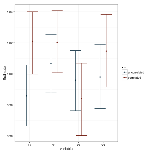
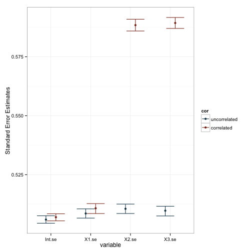
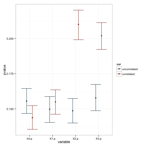
Well, it seems pretty clear that our manipulation lead to changes in the standard errors and, as a consequence, our pvalues. This is also reflected in the plot of the coefficients, as you can see that the variability in estimates is larger for X2 and X3 when they’re correlated. We can test these observations more formally with a series of linear models based on the data. Note that I dropped the intercept term in these models, and made X1 the baseline comparison group.
summary(lm(value~cor*variable, subset=variable!='Int', data=coefs))##
## Call:
## lm(formula = value ~ cor * variable, data = coefs, subset = variable !=
## "Int")
##
## Residuals:
## Min 1Q Median 3Q Max
## -2.34911 -0.35939 0.00165 0.35748 2.49402
##
## Coefficients:
## Estimate Std. Error t value Pr(>|t|)
## (Intercept) 1.006470 0.010859 92.684 <2e-16 ***
## corcorrelated 0.013900 0.015357 0.905 0.365
## variableX2 -0.010496 0.015357 -0.683 0.494
## variableX3 -0.008499 0.015357 -0.553 0.580
## corcorrelated:variableX2 -0.025657 0.021718 -1.181 0.237
## corcorrelated:variableX3 0.002798 0.021718 0.129 0.897
## ---
## Signif. codes: 0 '***' 0.001 '**' 0.01 '*' 0.05 '.' 0.1 ' ' 1
##
## Residual standard error: 0.543 on 14994 degrees of freedom
## Multiple R-squared: 0.0004957, Adjusted R-squared: 0.0001624
## F-statistic: 1.487 on 5 and 14994 DF, p-value: 0.1902summary(lm(value~cor*variable, subset=variable!='Int.se', data=se))##
## Call:
## lm(formula = value ~ cor * variable, data = se, subset = variable !=
## "Int.se")
##
## Residuals:
## Min 1Q Median 3Q Max
## -0.177621 -0.038599 -0.003009 0.035404 0.257936
##
## Coefficients:
## Estimate Std. Error t value Pr(>|t|)
## (Intercept) 0.508555 0.001108 458.824 <2e-16 ***
## corcorrelated 0.002201 0.001567 1.404 0.160
## variableX2.se 0.001990 0.001567 1.270 0.204
## variableX3.se 0.001180 0.001567 0.753 0.452
## corcorrelated:variableX2.se 0.075652 0.002217 34.127 <2e-16 ***
## corcorrelated:variableX3.se 0.077388 0.002217 34.910 <2e-16 ***
## ---
## Signif. codes: 0 '***' 0.001 '**' 0.01 '*' 0.05 '.' 0.1 ' ' 1
##
## Residual standard error: 0.05542 on 14994 degrees of freedom
## Multiple R-squared: 0.3111, Adjusted R-squared: 0.3108
## F-statistic: 1354 on 5 and 14994 DF, p-value: < 2.2e-16summary(lm(value~cor*variable, subset=variable!='Int.p', data=pvals))##
## Call:
## lm(formula = value ~ cor * variable, data = pvals, subset = variable !=
## "Int.p")
##
## Residuals:
## Min 1Q Median 3Q Max
## -0.2100 -0.1480 -0.1042 0.0580 0.8506
##
## Coefficients:
## Estimate Std. Error t value Pr(>|t|)
## (Intercept) 0.149763 0.004655 32.174 < 2e-16 ***
## corcorrelated 0.005193 0.006583 0.789 0.430
## variableX2.p -0.001104 0.006583 -0.168 0.867
## variableX3.p 0.008059 0.006583 1.224 0.221
## corcorrelated:variableX2.p 0.056176 0.009310 6.034 1.64e-09 ***
## corcorrelated:variableX3.p 0.038929 0.009310 4.182 2.91e-05 ***
## ---
## Signif. codes: 0 '***' 0.001 '**' 0.01 '*' 0.05 '.' 0.1 ' ' 1
##
## Residual standard error: 0.2327 on 14994 degrees of freedom
## Multiple R-squared: 0.01174, Adjusted R-squared: 0.01141
## F-statistic: 35.64 on 5 and 14994 DF, p-value: < 2.2e-16I hope this illustrates the importance of considering whether your predictors are correlated. Having correlated predictors results in a dramatic decrease in the precision of their estimates, which in turn influences the power to detect an effect. While this problem is not typically so great in experiments (as conditions feature random assignment), it can sometimes be a problem if the data are dramatically unbalanced, or if you are including a covariate in the model.
Furthermore, these few tutorial can serve as an illustration of the power of simulation as a method of investigation. In my view, there are few better ways to understand your data than to try to think of the process that generated it and seeing if your assumptions are correct by simulating that process. With the minimal examples I’ve used here, it should be possible to think of other parameters to adjust.