One powerful tool in an analyst’s toolbox is simulation. If you’re ever unsure about whether you can safely do some procedure or if modeling your data in a certain way is a good or bad idea, you can often get your answer through running a simulation. Unfortunately, I don’t think psychologists generally, receive the training needed to incorporate this into their workflow. That’s too bad, because it really is powerful. So, this is a primer on how to simulate. We’ll start with a relatively easy example. Before digging into the computation, however, we need to understand what it means to model data.

Statistical models

Suppose we run an experiment with a control group and an experimental group. If you read a statistics textbook, it will tell you that this can be described a model that takes the form of an equation like this:

Looks scary, right? There are latin letters, greek letters, and subscripts. What’s all that mean?

Well, \(y\) is the response, also known as the dependent variable. It’s the thing you’re looking to explain. You ran an experiment, and saw some outcome and you’re interested in what produced that outcome (hint - you manipulated some variable, right?). There’s a subscript to indicate that there are multiple instances of \(y\). In fact, if there are 4 observations of your dependent variable, then:

Let’s take a simple example. Here are your 4 observed values for \(y\)

y <- c(2, 4, 8, 10)
cat(y, sep='\n')

## 2
## 4
## 8
## 10

In this example, what is \(Y_i\) for \(i = 2\)? The way we access values in R works similarly to this notation. Let’s get \(Y_2\):

y[2]

## [1] 4

Now, we specified before that we ran an experiment with two groups. This is also represented in the equation above. Specifically, \(X\) will represent our manipulation. You’ll notice it is also denoted with a subscript \(i\), which means that it will have the same number of instances as there are in \(Y\). Since there are two groups, \(X\) will take on two values. There are a number of ways of representing these two groups numerically, but we’ll use 0 for control group and 1 for experimental group. Let’s return to our y variable. Which of these 4 observations came from the control group and which came from the experimental group?

cat(y, sep='\n')

## 2
## 4
## 8
## 10

We haven’t specified this until now, and it doesn’t really matter for this toy example which observation goes with which group. Because the latter two numbers of the \(Y\) vector are much larger, we’ll say that they came from the experimental group - this is what a big effect looks like!

Thus, that means that this is our x:

x <- c(0, 0, 1, 1)
cat(x, sep='\n')

## 0
## 0
## 1
## 1

So, we can plug these values into our equation above and we now have a series of equations that describe each outcome:

Now, we need to make these equations work mathematically. The objective is to find some values for \(\beta_0\) and \(\beta_{1}\) which will allow us to minimize the values for \(\epsilon\). Here, we’re not really worried about how the we arrive at the numbers that accomplish that, so I’m going to just approach this from an intuitive fashion.

First, we see that there are some spots where something is being multiplied by zero. That particular term, then, is zero, so let’s simplify:

Great, now we can try to find some good values to plug in here. Let’s first tackle $\beta_0$. This term is typically called the intercept or the constant. Because we have chosen to use a dummy code for \(X\) (i.e. zero and one), that means that the intercept is the value $Y$ takes when $X$ is zero. That means we’re looking at the values for \(Y_1\) and \(Y_2\). They aren’t identical, but taking their average is a pretty good way of describing them on the whole altogether. In this case, the average is 3, so let’s plug this into our system:

Next, we have \(\beta_1\). This is the term that indicates how much greater \(Y\) is for the experimental group than the control group. Taking a similar approach, we see that, in comparison to the average for the control group (3), the average for the experimental group (9) is 6 units higher. So, we can assign \(\beta_1\) a value of 6.

Simplifying that, we get:

The \(\epsilon\) term is called the error, or residuals. It’s the variance in y that we haven’t yet explained. The form of these residuals is very important for establishing that our quantitative description of the data (i.e. the equations we’re using - also known as the model) is a good one. For now, we’ll note that they should be normally distributed. In our toy example, they take the values:

resids <- c(-1, 1, -1, 1)
cat(resids, sep='\n')

## -1
## 1
## -1
## 1

Plugging those in, we see that we’ve solved the equations

Okay, so why did we go through all this trouble? Well, if we understand the way that these models work, then it makes it easy to generate fake data. Let’s do that.

Simulating data

First, let’s go back to the fake data we just used. We ended up deciding on a model that looks like this:

Where

And we said that our residuals were normally distributed. That implies that those residuals have a mean and some measure of variance. If we get the standard deviation of our residuals from above, we get:

sd(resids)

## [1] 1.155

which is really far too small. Psychological data are much noisier than that. Let’s use a more realistic number for our variability. We’ll have our residuals described as a normal distribution with a mean of zero (as it should always have) and a standard deviation of 10.

In other words, \(\epsilon \sim N(0, 10)\)

That epsilon term is key in letting us generate random data. Without it, we have a completely determined function that describes our dependent variable exactly:

So, it should be clear that we can generate some fake data by taking the following steps:

1. Decide how many individuals are in the control and how many are in the experimental group
2. Generate their perfectly determined data
3. Add some noise as described by the residuals

And here are those steps and a plot of the data:

set.seed(42) #for reproducibility
library(ggplot2)
#20 in each cell
X <- rep(c(0, 1), each=20)
#generate Y
Y <- 3 + 6*X
#add noise
Y <- Y + rnorm(40, 0, 10)

df <- data.frame(X=X, Y=Y)

ggplot(df, aes(x=Y)) +
  geom_density(aes(fill=factor(X)), alpha=.3) + 
  scale_fill_manual(values=c('#144256', '#88301B')) + 
  theme_bw()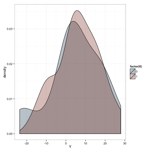

We’ve generated 20 observations in each of our groups. What do you think will happen if we fit a linear model to this simulated data?

m.1 <- lm(Y~X)
summary(m.1)

## 
## Call:
## lm(formula = Y ~ X)
## 
## Residuals:
##    Min     1Q Median     3Q    Max 
## -28.48  -4.86  -0.11   8.26  21.66 
## 
## Coefficients:
##             Estimate Std. Error t value Pr(>|t|)  
## (Intercept)     4.92       2.72    1.81    0.078 .
## X               1.37       3.84    0.36    0.723  
## ---
## Signif. codes:  0 '***' 0.001 '**' 0.01 '*' 0.05 '.' 0.1 ' ' 1
## 
## Residual standard error: 12.2 on 38 degrees of freedom
## Multiple R-squared:  0.00334,  Adjusted R-squared:  -0.0229 
## F-statistic: 0.127 on 1 and 38 DF,  p-value: 0.723

Remember what the underlying model was like for these data?

Where \(\epsilon_{i} \sim N(0, 10)\). However, the coefficients estimated from these data don’t look like that at all. Instead, we estimated the following underlying model:

What happened here? This is what happens when you’re dealing with really noisy measurements - your coefficients wont match the underlying generative model that well. However, we know that if we draw many samples from the same population, then the mean value of each of those samples will converge to the true population value. So, if we’ve done this correctly, we can simulate running many of these experiments, and we should see that the average across all of our experiments corresponds to the population values.

To do this, all we need to do is place the computations we just did in a loop such that they’re performed many times, making sure we save all the results.

#It's good practice to initialize any variables that would otherwise grow 
#inside the loop. It's easier for the computer to handle this way
coef.x <- numeric(1000)
coef.int <- numeric(1000)

#20 in each cell
X <- rep(c(0, 1), each=20)

#simulate the experiment 1000 times
for (i in 1:1000) {
  #generate Y
  Y <- 3 + 6*X
  #add noise
  Y <- Y + rnorm(40, 0, 10)
  
  df <- data.frame(X=X, Y=Y)
  
  m.1 <- lm(Y~X)
  coef.int[i] <- m.1$coefficients[1]
  coef.x[i] <- m.1$coefficients[2]
}

df <- data.frame(coefficient=c(coef.int, coef.x),
                 term=rep(c('intercept', 'x'), each=1000))

#dataframe indicating where the expected values lie
popvals <- data.frame(term=levels(df$term), coefficient=c(3, 6))

ggplot(df, aes(x=coefficient)) +
  geom_density(fill='#144256') + 
  facet_wrap(~term) +
  geom_vline(data=popvals, aes(xintercept=coefficient), color="#88301B") + 
  theme_bw()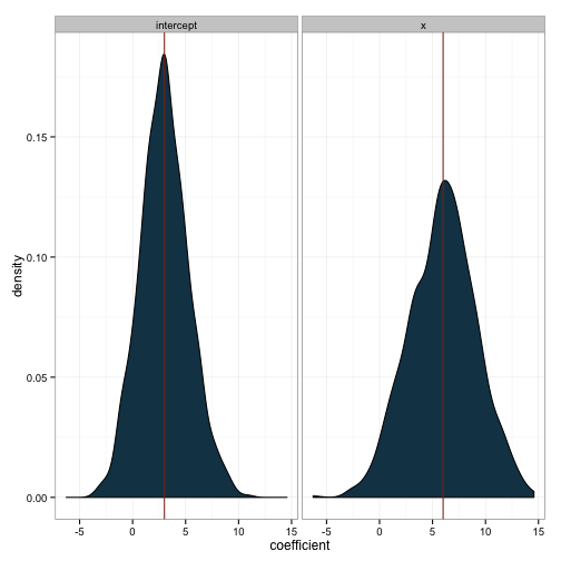

So, even though the first sample we drew was wildly inaccurate, we can see that our methods are valid. Now that we know how to use this tool, we can use it to answer substantive questions. We’ll see this in a future post.