The approach I have taken to simulation in this space so far has been pretty simple:

1. Set some values for the intercept and slope of a regression equation.
2. Generate the outcomes as a function of that equation.
3. Add some noise.

And voila - simulation!

However, sometimes we want to simulate something a little bit more complex. For instance, we may want to simulate data from a multivariate model in which some of the variables are correlated with each other in very specific ways. While the above approach will take you a long way, simulating these complex relationships would be very difficult using the simple methods I’ve been describing. Fortunately, we can use some alternative procedures to simulate data that fits these criteria.

For instance, let’s say that we want to generate some data that is a function of three continuous variables. Let’s further suppose that these three “predictor” variables are also correlated with each other. How can we do such a thing?

Well, it’s helpful in this case to understand the concept of a variance-covariance matrix. Using such a matrix, we can easily and flexibly specify how related we want our variables to be. For instance, if we have three variables, our variance-covariance matrix would look like this:

The variance for each variable lies along the diagonal, while the covariance between variables lie on the off-diagonal. We can see also that the matrix is symmetric, with the values below the diagonal mirrored by the values above the diagonal. For our purposes, we can use the scaled version of these measures, which means that the variance-covariance matrix is going to have 1’s along the diagonal and correlations on the off-diagonal.

Regardless, once we’ve generated our matrix, we can use it to constrain our randomly generated predictor variables to exhibit the properties of correlation that we’ve decided upon. R has great tools for accomplishing this.

First, let’s create our matrix. We’re going to have three variables - X, Y, and Z. X and Y will not be correlated, X and Z will be sligthly correlated, and Y and Z will be strongly correlated.

library(compiler)
library(corpcor)
library(MASS)

set.seed(42)
n<-100

#correlations between predictors
VCV <- matrix(c(1, 0, .2,
                0, 1, .7,
                .2, .7, 1), nrow=3, ncol=3)
rownames(VCV) <- c('X', 'Y', 'Z')
VCV

##   [,1] [,2] [,3]
## X  1.0  0.0  0.2
## Y  0.0  1.0  0.7
## Z  0.2  0.7  1.0

Great, having done this, we can use the mvrnorm function to turn this into observed variables. This function takes three arguments - the number of observations, the mean of each variable, and the matrix we just created and returns vectors of observations for each variable you’re generating. Here’s an example:

library(GGally)
library(ggplot2)
dat <- as.data.frame(mvrnorm(n = n, mu = rep(0, 3), Sigma = VCV))
ggpairs(dat, lower=list(params=c(color='#144256')), 
        diag=list(params=c(fill='#144256'))) + theme_bw()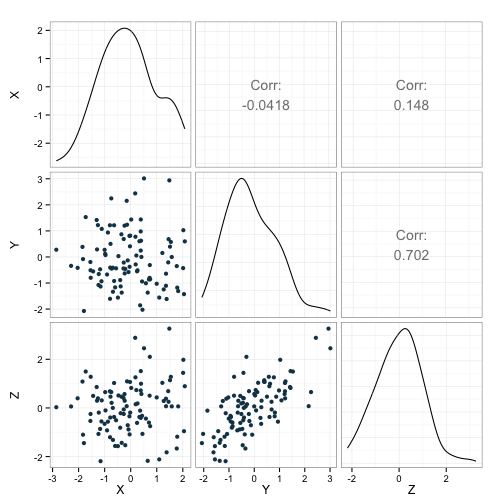

We can see that the correlation coefficients (indicated in the upper part of the figure) are in the neighborhood of what we wanted. This is further illustrated by the scatterplots in the lower bit of the figure.

We’ll continue with the series of posts on simulation next time, taking this approach a step or two closer to running a full simulation study.

This post was helped along considerably by a very instructive page on simulating multilevel data on the UCLA website.