We previously learned how to run a toy simulation. We described a straightforward linear model with an intercept and one slope parameter, generated some data, and found that if we simulated drawing data from the model described, the estimated slope and intercept converged onto the true values. That is, we saw no evidence of bias in our estimates. If the slope and intercept had converged to some values other than the ones we used to generate the data, then that would have indicated that our estimation methods were biased.

We can also use this tool to investigate questions of power. For instance, recall that the first model we fit to simulated data had coefficients that were much different. In fact, we were not able to reject the null hypothesis that the slope and intercept were different than zero (according to the generative model, they are). This happens because we’re dealing with noisy data and small sample sizes - a problem that plagues psychological research. This allows researchers to find evidence for effects that aren’t true (or at least aren’t as strong as they suggest), as well as to fail to find evidence for an effect that does exist (or suggest that the effect isn’t as strong as it really is). The technical language for these statistical phenomena are type I and type II errors respectively (incorrect conclusions about the strength of the evidence are sometimes referred to as type M errors).

So let’s say we run an experiment, and we see some difference between our groups. How often will that difference reach the level of statistical significance, given the set-up of our experiment?

Recall that we set up a model described as

Where \(\epsilon_{i} \sim N(0, 10)\)

Also recall that we had 20 participants in each group - this is one of the rules of thumbs that has been employed for a long time in psychology - at least 20 participants per cell. Let’s look at how often we can correctly reject the null under these conditions.

library(ggplot2)
library(reshape2)
library(dplyr)
#It's good practice to initialize any variables that would otherwise grow 
#inside the loop. It's easier for the computer to handle this way
coef.x <- numeric(1000)
p.x <- numeric(1000)
coef.int <- numeric(1000)
p.int <- numeric(1000)

#20 in each cell
X <- rep(c(0, 1), each=20)

#simulate the experiment 1000 times
for (i in 1:1000) {
  #generate Y
  Y <- 3 + 6*X
  #add noise
  Y <- Y + rnorm(40, 0, 10)
  
  df <- data.frame(X=X, Y=Y)
  
  m.1 <- lm(Y~X)
  coef.int[i] <- m.1$coefficients[1]
  p.int[i] <- summary(m.1)$coefficients[7]
  coef.x[i] <- m.1$coefficients[2]
  p.x[i] <- summary(m.1)$coefficients[8]
}

df <- data.frame(run = seq(1,1000),
                 coef.int=coef.int, coef.x=coef.x, p.int=p.int, p.x=p.x)
df.pvals <- melt(df, id.vars = 'run', measure.vars = c('p.int', 'p.x'))


power <- data.frame(variable=c('p.int', 'p.x'), proportion=prop.table(
  table(df.pvals$value<.05, df.pvals$variable), 2)[c(2, 4)])

ggplot(df.pvals, aes(x=value)) + 
  geom_density() + facet_wrap(~variable, scales='free')  + 
  geom_vline(aes(xintercept=.05), color="#88301B") + 
  geom_text(data=power, aes(x=Inf, y=Inf, label=paste('Power = ', proportion), 
                hjust=1.25, vjust=1.25)) + 
  theme_bw()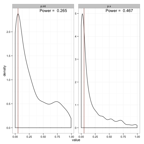

According to this method, we can see that we’ll correctly reject the null hypothesis that the intercept is zero only 26% of the time. The situation for the slope is a bit better - we’ll reject that one about 44% of the time. This clearly doesn’t reach the goal we usually shoot for (80%), but is probably pretty representative of the power of most psychological studies.

Let’s see what we can do about our power if we increase the number of individuals we recruit for our ‘studies’.

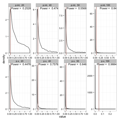
Along the top are the distributions of p-values for the intercept, while the bottom are the p-value distributions for the estimate of the slope. For the slope, which has a larger effect, we see that we need in the neighborhood of 50 observations in each cell to achieve a power of .80. The intercept, on the other hand, will require somewhere just under 100 obseervations per cell.

Learning the basic mechanics of simulation is a valuable skill. Anyone who works extensively with data should be able to do it, especially if you’re working in a frequentist framework.