This is a follow-up to my last set of notes on the hierarchical models I’ve been working with in stan for a while. I’m continuing the process of building it back up after tearing it down. Most of my work on this in the last couple of weeks has involved the exploration of strategies to remove divergent transitions from the hierarchical model I want to fit. Last time, I described a model in which observations were nested within individuals. I want to expand on that here. Now, there is additional structure. All observations have two additional nesting structures - the condition that the individual was in and the racial group they identify with. One of the nicest properties of a modeling language like stan is that if you have the coded model, you also exactly know the mathematical equivalent. So, I’ll forgo the tedious latex math (am I the only one that feels that way?) and instead just present the model. This is the simplest version, and the one I started with.

data {
  int<lower=1> n; //number of obs = 11212
  int<lower=1> p; //number of participants = 1174
  int<lower=1> conditions; //number of conditions = 2
  int<lower=1> group_conds; //number of race*condition combos = 10
  int c[group_conds]; //group condition indicator
  vector[n] y; // observed vals
  int s[p]; //number of obs per participant
  int sub_obs[n]; //subject observation indicator
  int race_cond[p]; //participant race_cond[p]

}
parameters {
  vector[p] b_mu; //mean for student p
  vector[group_conds] g_mu;
  vector[conditions] c_mu;
  vector<lower=0>[p] sigma_i; //variance for student p
  real<lower=0> sigma; //one grand sigma 
  real<lower=0> sigma_g;
  real<lower=0> sigma_c;
  real mu;  //sampled grand mean

}

model {
  int pos;
  mu ~ normal(2,1);
  sigma ~ normal(0,1);
  sigma_i ~ normal(0,1);
  sigma_g ~ normal(0,1);
  sigma_c ~ normal(0,1);
  c_mu ~ normal(mu, sigma);
  g_mu ~ normal(c_mu[c], sigma_c[c]);
  b_mu ~ normal(g_mu[race_cond], sigma_g[race_cond]);

  pos <- 1;
  for (i in 1:p){
    y[pos:pos+s[i]] ~ normal(b_mu[i], sigma_i[i]);
    pos <- pos+s[i];
  }
} 

So I’m estimating an overall mean, with the condition means estimated from that, and the race-condition group means estimated from those, followed by participants, then the data. You’ll notice that the prior for the overall mean is \(N(2,1)\). This basically gives good coverage to 0-4, and given that this is GPA data, that seems like an appropriate place to put the prior. I had initially had it at \(N(0,1)\), but that was giving a bunch of coverage to impossible values (negative GPA) and was pretty far from where the bulk of the data actually were (most students are between 2 and 4).

Running the above model leads to divergent transitions. The number varies from run-to-run, but usually it’s in the low hundreds. That’s not good. So how do you fix it? Well, the first step, according to the Stan manual, the rstan documentation, and most of the related posts on the stan-users mailing list is to look at a pairs() plot of some of the parameters. Of course, since there are over two thousand subject-level parameters alone (scale and location), we can’t look at all of them. Instead, we should pick a good collection of them from each level of the hierarchy. The purpose here is that we want to get a sense of what happens to as we move from one level of our hierarchical structure to another. Here’s the pairs plot for a small number of parameters, transformed on the log scale:

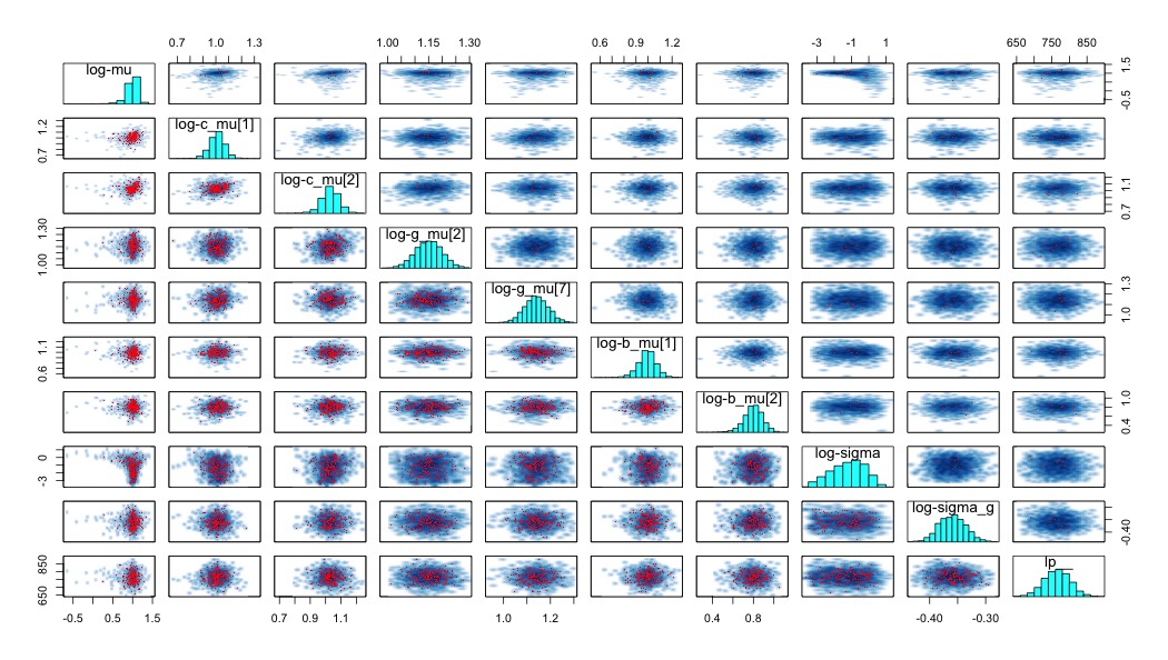
There’s a couple of things to notice here. First, most of the red dots (which represent divergent transitions) are in the lower triangular portion. These are the draws that are below the median acceptance probability. In a very helpful chain here, this is described as a situation in which there is a problem in the tails of the model. Furthermore, any parameters in which much of the mass is bunched up against some ‘wall’, or any pair of parameters that have unusual geometries that feature different variances along the range of values for one dimension can lead to sampling difficulties. I have an intuition of why this is, but I’m uncertain about how accurate this intuition is. Look at the plot of log-mu against log-sigma. Imagine creating a robot that is supposed to walk all over that space and get a good idea of it’s layout. The complication is that this robot can only take one very specific sized step from point to point. The size of that step that is appropriate to explore the log-mu dimension at log-sigma = -3 is not the same as at log-sigma = 0. This is why it’s difficult to sample from this type of structure.

Regardless of the accuracy of my intuition, in my case, both of those problems are present for the parameter mu (see the histogram in the top left corner and all associated scatter plots). Why might this be? Well, it’s important to note that this parameter is essentially being estimated with two data points - one for each of the two conditions. I don’t think it’s quite that simple, as these things are embedded in a bigger hierarchy, but that’s definitely been a recurring problem in other ways I’ve specified this model.

The solution I’ve used that appears to work well is to just remove that layer of the hierarchy. In truth, it was superflous anyway. If I want to shrink them toward some common value, I can just set that as the prior directly. Below, I’ve commented out that parameter and sampled c_mu directly from a normal distribution centered on 2

model {
  int pos;
  //mu ~ normal(2,1);
  sigma ~ normal(0,1);
  sigma_i ~ normal(0,1);
  sigma_g ~ normal(0,1);
  sigma_c ~ normal(0,1);
  c_mu ~ normal(2, sigma);
  g_mu ~ normal(c_mu[c], sigma_c);
  b_mu ~ normal(g_mu[race_cond], sigma_g);

  pos <- 1;
  for (i in 1:p){
    y[pos:pos+s[i]] ~ normal(b_mu[i], sigma_i[i]);
    pos <- pos+s[i];
  }
} 

That completely gets rid of the divergent transitions, and all the parameter estimates look reasonable. I should note that the one paper that exists on this problem mostly focuses on switching from centered to non-centered parameterization, and is the direction I pursued in the last post. Here, no combination of centered and/or un-centered parameters totally fixed the problem (though some combinations were certainly much worse!).

In addition to the links here, Gelman & Hill’s text on multilevel modeling was of considerable help with addressing these issues, especially chapters 12 and 13.