Previously, I examined how when calculating the standard deviation of a sample, if we divide by \(n\), we obtain a biased estimate. The problem is exacerbated when the sample size is small, as in the typical psychology experiment. To correct for this, one should instead divide by \(n - 1\). However, the more interesting question is what to do when you’re computing the standard deviation of two separate samples.

When performing a meta-analysis, you might take information from two samples, each of which may be characterized by its mean, standard deviation, and sample size. Combining means is relatively straightforward - just compute a weighted average. For standard deviation, my colleague found this suggestion to do a similar thing for standard deviation:

However, you’ll note that there’s no correction being applied here. Perhaps it’s taken care of, since each of these standard deviations is, presumably, itself the result of a correction. First, let’s draw a bunch of random samples from the same underlying population (M = 100, S = 10). Each sample will consist of 15-50 observations (uniformly distributed).

library(ggplot2)
library(reshape2)
set.seed(42)

numsamples <- 10000
mean <- 100
sd <- 10

simulation <- function(mean, sd, numsamples) {
  samples <- data.frame(mean.1=rep(0, numsamples), 
                        stdev.1=rep(0, numsamples),
                        n.1=round(runif(numsamples, 15, 50)),
                        mean.2=rep(0, numsamples),
                        stdev.2=rep(0, numsamples),
                        n.2=round(runif(numsamples, 15, 50)),
                        weighted_mean=rep(0,numsamples))
  
  for (i in 1:numsamples) {
    sample1 = rnorm(samples$n.1[i], mean, sd)
    sample2 = rnorm(samples$n.2[i], mean, sd)
    samples$mean.1[i] = mean(sample1)
    samples$mean.2[i] = mean(sample2)
    samples$stdev.1[i] = sd(sample1) #r uses the corrected version
    samples$stdev.2[i] = sd(sample2)
    samples$weighted_mean = weighted.mean(c(samples$mean.1[i], samples$mean.2[i]), c(samples$n.1[i], samples$n.2[i]))
  }
  
  return(samples)
}

samples<-simulation(mean, sd, numsamples)

Now, what happens if we take the simple weighted standard deviation, as described in the equation above?

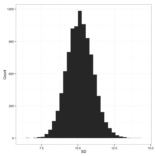
That looks pretty close. It’s slightly high, I suppose, at an average combined sd of 10.14. But there’s an inconsistency here. The wikipedia page which the above stack exchange answer links to gives a slightly modified formula (which I’ve rewritten slightly for consistency with the above equation:

Do you spot the difference? In the numerator, the sample standard deviations are weighted by \(n - 1\), while in the denominator the whole thing is divided by \(n_1 + n_2 - 1\). What’s this going to do to the combined standard deviation? It should make it slightly smaller. We’re effectively reducing the size of what’s in the numerator, which reduces the overall quantity, and reducing the size of what’s in the denominator, which has the same effect. Not coincidentally, the first method of calculation lead to a slight overestimation. What happens with the new method?

samples$weighted.sd.corrected <- with(samples, 
                 sqrt((((n.1-1)*stdev.1^2)+((n.2-1)*stdev.2^2)+
                         (n.1*((mean.1-weighted_mean)^2))+
                         (n.2*((mean.2-weighted_mean)^2)))/
                        (n.1+n.2-1)))

samples$calculation <- 1:numsamples
runs<-melt(samples, id.vars = 'calculation', measure.vars = c('weighted.sd', 
                                                              'weighted.sd.corrected'))
names(runs)[c(2,3)] <- c('method', 'standard_deviation')

plot <- ggplot(runs, aes(runs$method, runs$standard_deviation, 
                         fill=method))
plot + geom_boxplot() + 
  ylab('Standard Deviation') + xlab('Caclulation Method') + 
  theme_bw() + 
  theme(legend.position='none')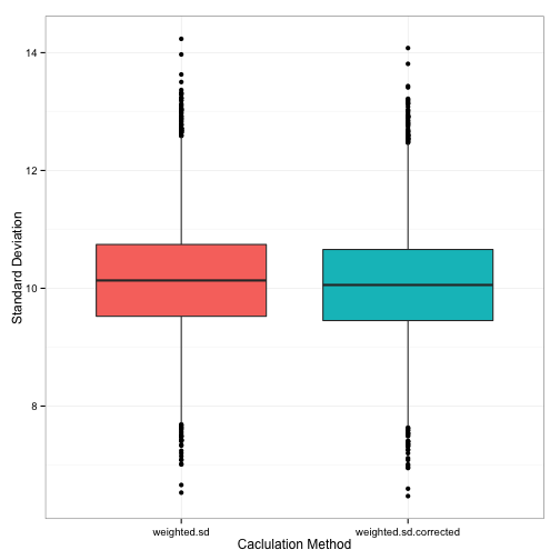

We get a slightly (very slightly) smaller combined standard deviation. But, happily enough, the average of all these standard deviations (10.06) is almost exactly lined up with what we know the population standard deviation to be (S = 10).