P-hacking reduces meta-analytic bias, but not as much as just running well-powered tests

Luke Sonnet recently sent me some analyses that suggested that p-hacking could reduce the bias present in a meta-analysis, given that there is publication bias in the literature. That analysis can be found here.

There has been plenty of ink spilled on how terrible p-hacking and publication bias are. However, indications that they could lead to positive outcomes (even if the positive outcome is contingent on the fact that something bad is happening in the first place), haven’t, to my knowledge, been discussed at all. I liked Luke’s approach, but felt that the scenarios he set up weren’t particularly realistic, at least for psychological research. The primary things I noted were as follows:

Even with Luke’s specified sample size of 400, I suspected that the power to detect the small effect he specified was quite low
Despite what I suspect to be a low-powered test, we don’t often see sample sizes of that size in psychology. Until recently, and perhaps still, the rule of thumb was to run 20 or 30 participants per cell. Since this is a one-celled design, we might expect someone to run about 20 or 30 people to explore the effect.
That sample size of 400 remained constant across all experiments within each scientific regime
I think a more common method of p-hacking in psychology is to run an additional few subjects, and recheck the analysis to see if it’s more favorable.

So I modified his analysis to explore these issues to see how the results would hold up. First, I look at how this work holds up when we modulate the sample sizes. Next, I explore a different variety of p-hacking. Whereas Luke simply simulated that the investigator who had a borderline p-value changed model specifications and was successful in phacking attempts 20% of the time, I did something a little different. First, I had each simulated experiment sample a randomly selected number of subjects between an upper and lower limit. Then, to explore the consequences of running some additional subjects, I simulated worlds in which investigators were willing to draw an additional 10 subjects up to two times or up to three times.

The other changes I made were to use loops instead of vectorized operations because I was having a hard time with the repeated adding subjects and testing, and reduce the number of simulations/experiments to save on the runtime. So the variability on all of these estimates is a little bit bigger, but I think it’s precise enough for my purposes

First, let’s refresh on Luke’s findings:

treat_pop <- rnorm(10^5, mean = 1, sd = 7)

# Function that takes a sample size and returns the mean and p-value
estimate_treat <- function(n) {
  samp <- sample(treat_pop, size = n)
  out <- t.test(samp)
  c(out$estimate, out$p.value, out$conf.int)
}

# Function to run n_exps experiments and compute a cumulative estimate under different
# scientific regimes.
cumulative_est <- function(n, n_exps, publication_bias, p_hacking_level, p_hacking_success) {
  experiment_estimates <- sapply(rep(n, n_exps), estimate_treat)
  ests <- experiment_estimates[1, ]
  pvals <- experiment_estimates[2, ]
  lower_bound <- experiment_estimates[3, ]
  
  # Find estimates that are able to be p-hacked
  phacked <- (pvals > 0.05 & (lower_bound + p_hacking_level) > 0)
  # Only a proportion of these succeed
  phacked_success <- (phacked & (cumsum(phacked) <= floor(sum(phacked) * p_hacking_success)))
  # Get the remaining insignificant estimates
  insignif <- (!phacked_success & pvals > 0.05)
  # Publish the first #insignificant * (1 - publication_bias)
  insignif_pub <- (insignif & (cumsum(insignif) <= floor(sum(insignif) * (1 - publication_bias))))
  
  # The published estaimates are all of the significant estimates, (1 - publication bias)
  # proportion of insignificant and non-p-hacked estimates, and p-hacked estimates
  
  # The p-hacked estimates are the original estimates + enough bias to get the lower bound
  # of the confidence interval to be just above 0.
  published_ests <- c(ests[pvals <= 0.05 | insignif_pub], ests[phacked_success] - lower_bound[phacked_success])
  
  return(mean(published_ests))
}

sims <- 250  
nobias.luke <- replicate(sims, cumulative_est(n = 400,
                                              n_exps = 500,
                                              publication_bias = 0,
                                              p_hacking_level = 0,
                                              p_hacking_success = 0))

pubbias.luke <- replicate(sims, cumulative_est(n = 400,
                                               n_exps = 500,
                                               publication_bias = 0.975,
                                               p_hacking_level = 0,
                                               p_hacking_success = 0))

pubbias_phack.luke <- replicate(sims, cumulative_est(n = 400,
                                                     n_exps = 500,
                                                     publication_bias = 0.975,
                                                     p_hacking_level = 0.2,
                                                     p_hacking_success = 0.95))


library(ggplot2)
library(reshape2)
plot.df <- melt(data.frame(nobias.luke, pubbias.luke, pubbias_phack.luke))

ggplot(plot.df, aes(x = value, fill = variable)) + 
  geom_density(alpha = 0.4) + 
  geom_vline(xintercept = 1) + 
  ggtitle("Meta-Analysis Parameter Estimates\n under Different Publication Behaviors") + 
  xlab("Cumulative Parameter Estimate") +
  theme_bw() + 
  scale_fill_manual(values = c('#88301B', '#4F7C19', '#144256'))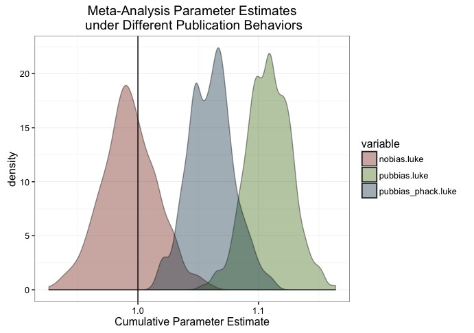

Got it? Publication bias is bad. P-hacking can reduce the severity of bad.

Power

The first thing to expore is what the power/sample size dynamic is here? The effect size is \(\frac{1}{7} = .14\). To reliably detect an effect that small with power of .8, you’re gonna need a bigger sample than 400. How much bigger?

library(pwr)

big <- pwr.t.test(d=1/7, sig.level=.05, power=.8)

floor(big$n)

## [1] 770

Yeah, nearly 800. Fortunately, this is not so difficult, because we’re just doing this through simulation. We just need to change a couple of numbers to get our desired sample size. Below, we see what happens when we use a sample size of 770 - enough for power of .80.

nobias.luke2 <- replicate(sims, cumulative_est(n = 770,
                                         n_exps = 500,
                                         publication_bias = 0,
                                         p_hacking_level = 0,
                                         p_hacking_success = 0))

pubbias.luke2 <- replicate(sims, cumulative_est(n = 770,
                                          n_exps = 500,
                                          publication_bias = 0.975,
                                          p_hacking_level = 0,
                                          p_hacking_success = 0))

pubbias_phack.luke2 <- replicate(sims, cumulative_est(n = 770,
                                                n_exps = 500,
                                                publication_bias = 0.975,
                                                p_hacking_level = 0.2,
                                                p_hacking_success = 0.95))

plot.df <- melt(data.frame(nobias.luke2, pubbias.luke2, pubbias_phack.luke2))

ggplot(plot.df, aes(x = value, fill = variable)) + 
  geom_density(alpha = 0.4) + 
  geom_vline(xintercept = 1) + 
  geom_vline(xintercept = mean(pubbias.luke), linetype='longdash') +
  ggtitle("Meta-Analysis Parameter Estimates\n under Different Publication Behaviors\n Large Samples") + 
  xlab("Cumulative Parameter Estimate") +
  theme_bw() + 
  scale_fill_manual(values = c('#88301B', '#4F7C19', '#144256'))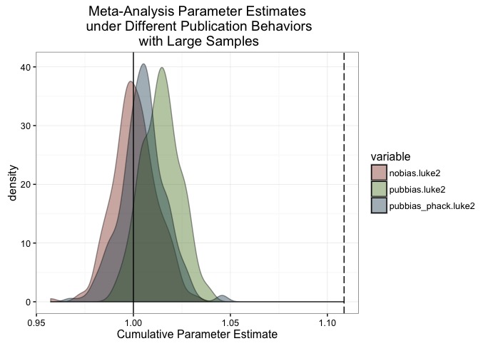

Huh! looks like all of our problem nearly disappears! Obviously there’s still some bias there (bias should be measured as distance from the distribution with no bias), but it’s pretty miniscule. The dotted line serves as a reference - it’s the estimated mean of from the first plot. That is, publication bias when all the experiments have an n of 400.

So, given this simplified scientific world, if people just ran studies that were appropriately powered, there wouldn’t be much of a problem with meta-analyses overestimating effects, even if there was publication bias. Unfortunately, figuring out the appropriate sample size is basically an impossible task, because no one knows what effect size they’re studying, and even small differences in the effect size can lead to huge changes in the sample needed to reliably study it.

Variable sample size & running extra subjects

So given that, let’s see what happens under some variants of the setup above. First, let’s explore with a range of values that are roughly on par with the original sample size of 400.

#Gets the subjects for a single study
exp_dat <- function(nmin, nmax){
  n = floor(runif(1, nmin, nmax))
  samp <- sample(treat_pop, size = n)
  return(samp)
}

# Function that takes sample and returns the mean and p-value
estimate_treat <- function(samp) {
  out <- t.test(samp)
  c(out$estimate, out$p.value, out$conf.int)
}



# Function to run n_exps experiments and compute a cumulative estimate under different
# scientific regimes.
cumulative_est <- function(nmin, nmax, n_exps, addl_sub_iters, pub_bias) {
  out <- rep(NA, n_exps)
  for(i in 1:n_exps){
    dat <- exp_dat(nmin, nmax)
    results <- estimate_treat(dat)
    j=0
    if (results[2] >.05){
      while(j < addl_sub_iters){
        dat <- c(dat, exp_dat(10,10))
        results <- estimate_treat(dat)
        if (results[2]<.05) break
        j=j+1
      }
    }
    if(results[2] < .05){
      out[i] <- results[1]
    }else{
      if(runif(1) > pub_bias){
        out[i] <- results[1]
      }
    }
  }
  return(mean(out, na.rm=T))
}

nobias <- replicate(sims, cumulative_est(nmin=375,
                                         nmax=425, 
                                         n_exps=500, 
                                         addl_sub_iters = 0, 
                                         pub_bias = 0))
pubbias <- replicate(sims, cumulative_est(nmin=375,
                                          nmax=425, 
                                          n_exps=500, 
                                          addl_sub_iters = 0, 
                                          pub_bias = .975))
pubbias_phack_2iter <- replicate(sims, cumulative_est(nmin=375,
                                                      nmax=425, 
                                                      n_exps=500, 
                                                      addl_sub_iters = 2, 
                                                      pub_bias = .975))
pubbias_phack_3iter <- replicate(sims, cumulative_est(nmin=375,
                                                      nmax=425, 
                                                      n_exps=500, 
                                                      addl_sub_iters = 3, 
                                                      pub_bias = .975))


plot.df <- melt(data.frame(nobias, pubbias, pubbias_phack_2iter, pubbias_phack_3iter))

ggplot(plot.df, aes(x = value, fill = variable)) + 
  geom_density(alpha = 0.4) + 
  geom_vline(xintercept = 1) + 
  geom_vline(xintercept = mean(pubbias.luke), linetype='longdash') +
  ggtitle("Meta-Analysis Parameter Estimates\n when investigators data peek") + 
  xlab("Cumulative Parameter Estimate") +
  theme_bw() + 
  scale_fill_manual(values = c('#88301B', '#136233', '#144256', '#88551B'))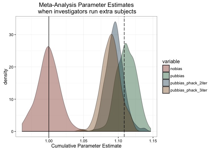

As you can see, the basic problem is still there - publication bias will lead to biases in metanalytic effect estimates. However, if the only way our investigators p-hack is through running additional subjects, then it would take quite a lot of work to get the effect down to the point at which Luke was observing.

The pattern persists for tiny (but more psychologically accurate) sample sizes. Unsurprisingly, running extra subjects at such small sample sizes moves the needle a little bit more.

nobias2 <- replicate(sims, cumulative_est(nmin=50,
                                         nmax=100, 
                                         n_exps=500, 
                                         addl_sub_iters = 0, 
                                         pub_bias = 0))
pubbias2 <- replicate(sims, cumulative_est(nmin=50,
                                          nmax=100, 
                                          n_exps=500, 
                                          addl_sub_iters = 0, 
                                          pub_bias = .975))
pubbias_phack_2iter2 <- replicate(sims, cumulative_est(nmin=50,
                                                      nmax=100, 
                                                      n_exps=500, 
                                                      addl_sub_iters = 2, 
                                                      pub_bias =.975))
pubbias_phack_3iter2 <- replicate(sims, cumulative_est(nmin=50,
                                                      nmax=100, 
                                                      n_exps=500, 
                                                      addl_sub_iters = 3, 
                                                      pub_bias = .975))
kable(matrix(c(1, mean(nobias2), mean(pubbias2), mean(pubbias_phack_2iter2),
               mean(pubbias_phack_3iter2)), nrow = 1, 
             dimnames = list(NULL, c("True parameter", "No bias", "Pub. bias", 
                                     "Pub bias + p-hacking - 2 rounds",
                                     "Pub bias + p-hacking - 3 rounds"))),
      digits = 2)

plot.df <- melt(data.frame(nobias2, pubbias2, pubbias_phack_2iter2, pubbias_phack_3iter2))

ggplot(plot.df, aes(x = value, fill = variable)) + 
  geom_density(alpha = 0.4) + 
  geom_vline(xintercept = 1) + 
  geom_vline(xintercept = mean(pubbias.luke), linetype='longdash') +
  ggtitle("Meta-Analysis Parameter Estimates\n when investigators data peek") + 
  xlab("Cumulative Parameter Estimate") +
  theme_bw() + 
  scale_fill_manual(values = c('#88301B', '#136233', '#144256', '#88551B'))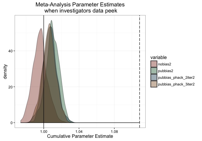

Finally, we see, once again, that when we use sample sizes that are roughly on par with the power required to detect this effect, that all of our problems disappear.

sims <- 250   
nobias3 <- replicate(sims, cumulative_est(nmin=750,
                                         nmax=800, 
                                         n_exps=500, 
                                         addl_sub_iters = 0, 
                                         pub_bias = 0))
pubbias3 <- replicate(sims, cumulative_est(nmin=750,
                                          nmax=800, 
                                          n_exps=500, 
                                          addl_sub_iters = 0, 
                                          pub_bias = .975))
pubbias_phack_2iter3 <- replicate(sims, cumulative_est(nmin=750,
                                                      nmax=800, 
                                                      n_exps=500, 
                                                      addl_sub_iters = 2, 
                                                      pub_bias =.975))
pubbias_phack_3iter3 <- replicate(sims, cumulative_est(nmin=750,
                                                      nmax=800, 
                                                      n_exps=500, 
                                                      addl_sub_iters = 3, 
                                                      pub_bias = .975))


plot.df <- melt(data.frame(nobias3, pubbias3, pubbias_phack_2iter3, pubbias_phack_3iter3))

ggplot(plot.df, aes(x = value, fill = variable)) + 
  geom_density(alpha = 0.4) + 
  geom_vline(xintercept = 1) + 
  geom_vline(xintercept = mean(pubbias.luke), linetype='longdash') +
  ggtitle("Meta-Analysis Parameter Estimates\n when investigators data peek") + 
  xlab("Cumulative Parameter Estimate") +
  theme_bw() + 
  scale_fill_manual(values = c('#88301B', '#136233', '#144256', '#88551B'))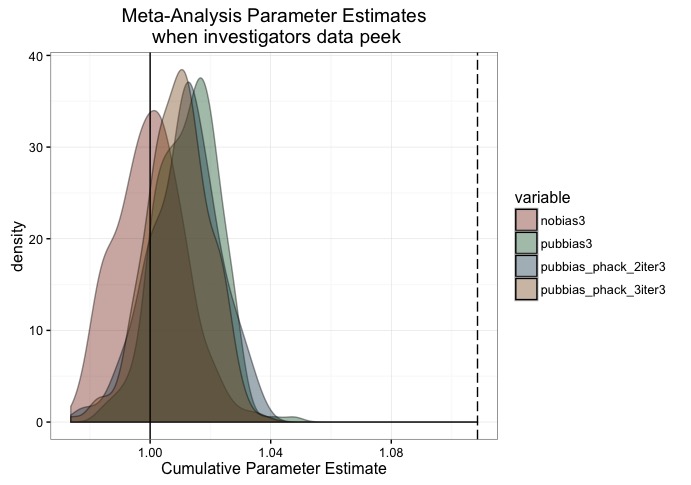

There are a couple of take-aways from this, I think. First is that, in principle, using the correct sample size for whatever effect you’re studying is of paramount importance. An appropriate sample size can resolve many issues, including those highlighted here. Unfortunately, as highlighted by others, getting a good estimate of effect size is difficult. Even more difficult is knowing how variable your estimate is, and thus, how many participants to shoot for. For a discussion of these problems, Joe Simmons and Uri Simonsohn have a nice series of posts on this, though for a somewhat more positive spin, see Jake Westfall’s post here.

Second, it seems clear that p-hacking can lead to a reduction in meta-analytic bias. A key question, though, is what the size of this effect would be in the population. This question is not going to be easy to answer, as you’ll need an estimate of how hard people have worked to p-hack, how power varies from study-to-study, field-to-field, and discipline-to-discipline, and the scale of publication bias.

Finally, I’d like to think that the importance of all this is quickly diminishing. Hopefully people have gotten the message that there are some issues in the way we have been conducting and communicating our science, and are working hard to alleviate the issues within their own work, as well as across science more widely. Maybe I’m overly optimistic here, though.

Luke Responds

I sent a draft of this to Luke to get his thoughts. They’re pasted below:

I think you’re totally right about everything you say. The numbers I chose were explicitly to make the point that this counter-intuitive result is possible in some scenarios. In reality, there are many ways that publication bias and p-hacking affect results. Indeed, p-hacking could be focusing on one of a set of parameters, adding small numbers of new observations (although this is far less likely in political science than psychology, I would imagine), changing model specifications, and more.

However, I think your main argument here is that these problems go away with well-powered tests. I obviously agree with that, however the problem is I don’t think we live in that world.

Written on February 29, 2016