I’ve been working on a particular statistical model for a while now. I’m doing the fitting using stan. It took a while to build the model up to the point where I was answering interesting research questions, but now I’m tearing it back down because there are some things going on that I don’t understand. What follows is mostly a set of notes to myself on the results of some simple experimentation on different ways of specifying the same model.

At the simplest, I’ve got close to 9000 observations of student grades that I can describe with a grand mean. In stan, that looks like this:

data {
  int<lower=1> n; //number of obs
  vector[n] y; // observed vals
}

parameters {
  real<lower=0> sigma; //one grand sigma 
  real mu
}

model {
  y ~ normal(mu, sigma);
}

No surprisingly, that works. The three chains (2000 iterations, with 1000 warmup draws) run in a total of about 1 second. The mean is estimated (using the median of the posterior) at 2.72, with the 95% credible intervals extending from 2.69-2.74. As you would expect with that many observations, the estimate is pretty darn precise.

(Un)fortunately, the structure of these data is a little more complicated than that. Those 9000 grades come from about 1200 students. Multiple grades per person = hierarchical structure. The gist of what we want to do is estimate a mean for each student, and then use the student estimates to inform an overall estimate. Expressed formally:

In stan, I’ve written this model in a couple of different ways to check how performance differs. Model 1:

data {
  int<lower=1> n; //number of obs
  int<lower=1> p; //number of participants
  vector[n] y; // observed vals
  int s[p]; //number of obs per participant
  int sub_obs[n]; //subject observation indicator
}
parameters {
  vector[p] b_mu; //mean for student p
  vector<lower=0>[p] sigma_i; //variance for student p
  real mu_raw;  //sampled grand mean

  real<lower=0> mu_scaler;
  real<lower=0> b_mu_scaler;

}
transformed parameters {
  vector[p] p_mu; //matt tricked mean for student p
  real mu; //matt tricked grand mean

  mu <- mu_raw * mu_scaler;
  p_mu <- mu + b_mu*b_mu_scaler;
}

model {
  int pos;
  mu_raw ~ normal(0,1);
  mu_scaler ~ normal(0,1);

  sigma_i ~ normal(0,1);
  b_mu ~ normal(0, 1); // implies ~ normal(mu, 1)

  pos <- 1;
  for (i in 1:p){
  	y[pos:pos+s[i]] ~ normal(p_mu[i], sigma_i[i]);
    pos <- pos+s[i];
  }
}

So, a bit hairier than the mean-only model, but still not too bad. I’m estimating an overall mean (mu) by first estimating its location on a unit normal distribution (mu_raw), and then scaling it to the place on the scale of the data (mu_scaler). I do the same thing for the individual subject means (b_mu). This is known as a non-centered parameterization. Also sometimes called the ‘Matt Trick’, after Matt Hoffman (see section 21.2 of the Stan manual). You’ll also notice there’s this new loop: for (i in 1:p){...}. That’s to take care of the different number of observations from each person (a slight improvement on the technique I described here).

This works to a degree. The estimates are on par with what we would expect given the simpler model above (M = 2.74, credibility interval = 2.68-2.79). It does take a bit longer to run at just under 10 minutes per chain (I’m not running in parallel). That’s not such a big deal. Time to run, I can deal with. What’s not so great are these warning messages:

Warning messages:
1: There were 15 divergent transitions after warmup. Increasing adapt_delta above 0.8 may help. 
2: There were 796 transitions after warmup that exceeded the maximum treedepth. Increase max_treedepth above 10. 
3: Examine the pairs() plot to diagnose sampling problems

These are issues that have to do with the way Stan’s sampling methodology. These problems can indicate problems with the results. The details of this are pretty technical, and pretty far out of my comfort zone, but suffice to say that you should not have any divergent transitions, nor any that exceed the maximum treedepth. So, trying a different parameterization:

data {
  int<lower=1> n; //number of obs
  int<lower=1> p; //number of participants
  vector[n] y; // observed vals
  int s[p]; //number of obs per participant
  int sub_obs[n]; //subject observation indicator
}
parameters {
  vector[p] b_mu; //mean for student p
  vector<lower=0>[p] sigma_i; //variance for student p
  real<lower=0> sigma; //one grand sigma 
  real mu;  //sampled grand mean

}

model {
  int pos;
  mu ~ normal(0,1);
  sigma_i ~ normal(0,1);
  b_mu ~ normal(mu, sigma);

  pos <- 1;
  for (i in 1:p){
    y[pos:pos+s[i]] ~ normal(b_mu[i], sigma_i[i]);
    pos <- pos+s[i];
  }
}

I’ve switched to a centered parameterization. I had initially used the non-centered parameterization because in the manual and in the Stan users mailing list, the non-centered parameterization is supposed to help with hierarchical models. However, it turns out that in this case, using the centered parameterization improves the speed substantially, running in under a minute. We also don’t see any of those pesky warning messages. The estimates are right in line with what’s expected too (M = 2.74, credibility interval = 2.68-2.79). Why is the centered parameterization better here? Bob Carpenter has a good writeup of this here, but I suspect that this is because I have a good amount of data. There are 900 “groups’ here that I’m estimating underneath the overall mean mu. If there were, say, 4 groups, then the non-centered might be preferable.

Because this model is dead-simple, I can also give rstanarm a whirl to see what it does with these data.

m.rstanarm <- stan_glmer(overallgpa_qtr ~ 1 + (1|ID), data=df.mod, prior_intercept=normal(0,1))

I’ve manually specified the prior on the intercept to make it a bit more equivalent with the models I’ve coded. I was kind of surprised that this took a bit longer than the last model at an average of about 6 minutes per chain. I also got a slightly different estimate for the value of the intercept (M = 2.68, 2.63-2.74). I’m inclined to think that the faster model I coded up above is preferable for a couple of reasons. First, it’s faster. Second, and more importantly, there’s pretty high autocorrelation for the draws from the posterior for estimating the intercept in rstanarm. For with 4000 independent draws, I’ve only got an effective sample size of 160 (.04%), and an \(\hat{R}\) of 1.02 . In contrast, with the model I coded up above, I get 3000 independent draws, with an \(\hat{R}\) of 1. The difference is pretty clearly visible in the traceplots too:

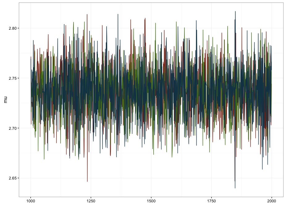Figure 1: Artisinal, hand-coded model

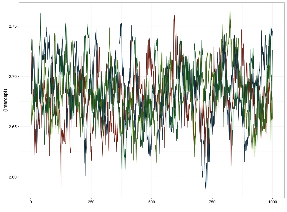
Figure 2: Mass-produced model

There’s nothing else fishy going on with my model either. At least, none that I’ve found. I should point out that this business about artisinal vs. mass-produced is done in jest. Clearly Stan and the affiliated products and packages are an incredible research tool, and we’re lucky to have people who have worked so hard on them. To be honest, I’m surprised that what I’ve coded can stack up against what these folks have produced. Next step is to scale it up to something a little more interesting.