
Speeding Things Up
I recently found a pretty interesting dataset I thought I’d examine a little bit. I took the following data from menustat.org. You can easily download the same data by using their ‘search’ function, and having it return all data for all available years. Once done, there’s a button that lets you export the data as a csv.
The size of this dataset also means that there were some pieces that I wrote off the cuff which turned out to be far too slow. Changing things around a little bit resulted in a substantial speed-up. I’ll take us through some data prep and then show two pieces of code that do the same thing, one of which operates significantly faster. Typically, I don’t deal with datasets where thinking about speed-up offers much payoff - everything runs fast when you’re only dealing with 150 observations. In fact, I’ve previously mentioned how this idea of “powerful” code is something I’m not too concerned about. However, due to size, the present case is a bit different.
Read the data
menus<-read.csv('../Data/menustat-546cf6b433804.csv')
#this doesn't work.  Throws an error:

#Error in read.table(file = file, header = header, sep = sep, quote = quote,  :
#  more columns than column names
Aw damn. Well, that didn’t work. Why not? The error message says that there’s a mismatch between the number of columns, and the number of names it has for the columns. Usually, this function reads the column names from the first line of the csv document, so I’m guessing that something is wrong with the first line of the csv. Opening it up in a text editor shows the following:
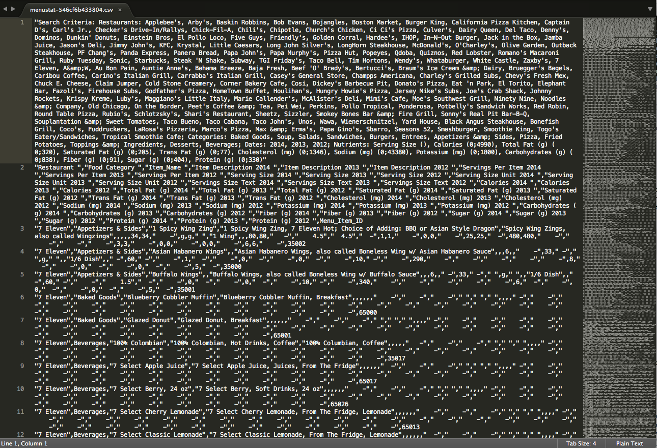
See the big chunk of text next to the 1 on the lefthand side? That’s all the stuff that appears in the first line, and we can see that it’s just kind of a description of the file. We can get rid of that. Line 2 seems to have the columns we want. While we’re at it, we can also see that there’s a bunch of empty cells that look like this: “ -“. When we read this into r, it will be represented as ‘\t-‘. There are also some spots where there’s a tab without the dash (i.e. ‘ ‘). We’re gonna get rid of those too. So we’re going to take a slightly different approach from just reading in the csv:
- Read the file, line by line as one big vector
- Remove the first line.
- Replace any ‘ -‘ or ‘ ‘ with a simple blank cell.
- Turn the vector into a dataframe.
menus<-readLines('../Data/menustat-546cf6b433804.csv')
menus<-menus[-1]
menus<-gsub('\t-', '', menus)
menus<-gsub('\t', '', menus)
system.time(menus<-read.csv(textConnection(menus)))
## user system elapsed
## 59.730 0.090 59.967That last line takes a while - about a full minute on my desktop machine. If there’s a way to speed that up, I don’t know it. At any rate, now we’ve got a big, beautiful datafile for our menus data! Let’s get some information about it:
dim(menus)## [1] 60238 52We’ve got 60,238 observations across 52 different variables. Let’s get a little information about those variables.
str(menus)## 'data.frame': 60238 obs. of 52 variables:
## $ Restaurant. : Factor w/ 150 levels "7 Eleven","A&W",..: 1 1 1 1 1 1 1 1 1 1 ...
## $ Food.Category. : Factor w/ 12 levels "Appetizers & Sides",..: 1 1 1 2 2 3 3 3 3 3 ...
## $ Item_Name. : Factor w/ 53247 levels "'Rita Trio","'Shroom & Swiss Sandwich",..: 602 3100 7417 6208 20871 854 1688 1689 1690 1691 ...
## $ Item.Description.2014. : Factor w/ 45533 levels "","'Rita Trio, Margaritas",..: 584 1 1 5474 19108 801 1463 1464 1465 1466 ...
## $ Item.Description.2013. : Factor w/ 42069 levels "","'Rita Trio",..: 36027 2268 5619 1 1 655 1 1 1 1 ...
## $ Item.Description.2012. : Factor w/ 15380 levels "","'Rita Trio",..: 1 1 1 1 1 1 1 1 1 1 ...
## $ Servings.Per.Item.2014. : Factor w/ 18 levels "","'4-6","10",..: 1 1 1 1 1 1 1 1 1 1 ...
## $ Servings.Per.Item.2013. : Factor w/ 22 levels "","'4-6","'5-6",..: 1 19 19 1 1 1 1 1 1 1 ...
## $ Servings.Per.Item.2012. : num NA NA NA NA NA NA NA NA NA NA ...
## $ Serving.Size.2014. : Factor w/ 1132 levels "","<1","0","0.3",..: 486 1 1 1 1 1 1 1 1 1 ...
## $ Serving.Size.2013. : Factor w/ 1083 levels "","<1","0","0.7",..: 467 449 449 1 1 1 1 1 1 1 ...
## $ Serving.Size.2012. : Factor w/ 682 levels "","<1","0.7",..: 1 1 1 1 1 1 1 1 1 1 ...
## $ Serving.Size.Unit.2014. : Factor w/ 6 levels " ","fl oz","fl oz*",..: 4 1 1 1 1 1 1 1 1 1 ...
## $ Serving.Size.Unit.2013. : Factor w/ 6 levels " ","fl oz","fl oz*",..: 4 4 4 1 1 1 1 1 1 1 ...
## $ Serving.Size.Unit.2012. : Factor w/ 6 levels " ","fl oz","fl oz*",..: 1 1 1 1 1 1 1 1 1 1 ...
## $ Servings.Size.Text.2014.: Factor w/ 385 levels "","0.25 Cup",..: 148 1 1 1 1 1 1 1 1 1 ...
## $ Servings.Size.Text.2013.: Factor w/ 168 levels "","0.25 Cup",..: 1 87 87 1 1 1 1 1 1 1 ...
## $ Servings.Size.Text.2012.: Factor w/ 159 levels "","1 Bag","1 Biscuit",..: 1 1 1 1 1 1 1 1 1 1 ...
## $ Calories.2014. : Factor w/ 1958 levels "","<5","0","0-10",..: 1723 1 1 1 1 1 1 1 1 1 ...
## $ Calories.2013. : Factor w/ 2415 levels "","<1","<5","0",..: 2124 1802 1802 1 1 1 1 1 1 1 ...
## $ Calories.2012. : Factor w/ 1166 levels "","<5","0","0-10",..: 1 1 1 1 1 1 1 1 1 1 ...
## $ Total.Fat..g..2014. : Factor w/ 606 levels "","<1",">1","0",..: 389 1 1 1 1 1 1 1 1 1 ...
## $ Total.Fat..g..2013. : Factor w/ 1038 levels "","<1","0","0-0.5",..: 718 74 97 1 1 1 1 1 1 1 ...
## $ Total.Fat..g..2012. : Factor w/ 405 levels "","0","0-1","0-22",..: 1 1 1 1 1 1 1 1 1 1 ...
## $ Saturated.Fat..g..2014. : Factor w/ 373 levels "","<1",">1","0",..: 38 1 1 1 1 1 1 1 1 1 ...
## $ Saturated.Fat..g..2013. : Factor w/ 346 levels "","<1","0","0-5",..: 36 3 3 1 1 1 1 1 1 1 ...
## $ Saturated.Fat..g..2012. : Factor w/ 230 levels "","0","0-4.5",..: 1 1 1 1 1 1 1 1 1 1 ...
## $ Trans.Fat..g..2014. : Factor w/ 121 levels "","<0.1","<0.2",..: 7 1 1 1 1 1 1 1 1 1 ...
## $ Trans.Fat..g..2013. : Factor w/ 127 levels "","<0.1","<0.2",..: 30 30 30 1 1 1 1 1 1 1 ...
## $ Trans.Fat..g..2012. : Factor w/ 52 levels "","<0.1","<0.2",..: 1 1 1 1 1 1 1 1 1 1 ...
## $ Cholesterol..mg..2014. : Factor w/ 937 levels "","<1","<5",">1",..: 310 1 1 1 1 1 1 1 1 1 ...
## $ Cholesterol..mg..2013. : Factor w/ 1188 levels "","<1","<5","0",..: 436 47 47 1 1 1 1 1 1 1 ...
## $ Cholesterol..mg..2012. : Factor w/ 529 levels "","<5","0","0-20",..: 1 1 1 1 1 1 1 1 1 1 ...
## $ Sodium..mg..2014. : Factor w/ 3281 levels "","<5",">25",..: 2448 1 1 1 1 1 1 1 1 1 ...
## $ Sodium..mg..2013. : Factor w/ 3642 levels "","<1","<5","0",..: 2711 1951 2228 1 1 1 1 1 1 1 ...
## $ Sodium..mg..2012. : Factor w/ 1772 levels "","0","0-100",..: 1 1 1 1 1 1 1 1 1 1 ...
## $ Potassium..mg..2014. : int NA NA NA NA NA NA NA NA NA NA ...
## $ Potassium..mg..2013. : int NA NA NA NA NA NA NA NA NA NA ...
## $ Potassium..mg..2012. : int NA NA NA NA NA NA NA NA NA NA ...
## $ Carbohydrates..g..2014. : Factor w/ 859 levels "","<1",">1","0",..: 467 1 1 1 1 1 1 1 1 1 ...
## $ Carbohydrates..g..2013. : Factor w/ 1301 levels "","<1","0","0-15",..: 665 1219 1062 1 1 1 1 1 1 1 ...
## $ Carbohydrates..g..2012. : Factor w/ 471 levels "","<1","0","0-1",..: 1 1 1 1 1 1 1 1 1 1 ...
## $ Fiber..g..2014. : Factor w/ 210 levels "","<0.5","<1",..: 6 1 1 1 1 1 1 1 1 1 ...
## $ Fiber..g..2013. : Factor w/ 479 levels "","<0.5","<1",..: 4 4 4 1 1 1 1 1 1 1 ...
## $ Fiber..g..2012. : Factor w/ 121 levels "","<1","<2","0",..: 1 1 1 1 1 1 1 1 1 1 ...
## $ Sugar..g..2014. : Factor w/ 586 levels "","<1",">1","0",..: 4 1 1 1 1 1 1 1 1 1 ...
## $ Sugar..g..2013. : Factor w/ 433 levels "","<1","0","0-17",..: 3 3 3 1 1 1 1 1 1 1 ...
## $ Sugar..g..2012. : Factor w/ 327 levels "","<1","0","0-1",..: 1 1 1 1 1 1 1 1 1 1 ...
## $ Protein..g..2014. : Factor w/ 504 levels "","<1",">1","0",..: 403 1 1 1 1 1 1 1 1 1 ...
## $ Protein..g..2013. : Factor w/ 1003 levels "","<1","0","0-1",..: 800 731 731 1 1 1 1 1 1 1 ...
## $ Protein..g..2012. : Factor w/ 356 levels "","<1","0","0-2",..: 1 1 1 1 1 1 1 1 1 1 ...
## $ Menu_Item_ID : int 35002 35000 35001 65000 65001 35017 65017 65026 65013 65012 ...We can now see the names for our variables. Looks like there’s one for restaurant, one for food category, one for the item, and then we have a bunch of variables which are repeated for each of 3 years: 2014, 2013, 2012. These variables describe the item, give us a serving size, and then the nutrient information (e.g. calories, fat, carbs, protein, etc.). We can also see that everything, with a couple of exceptions, is stored as a factor, which isn’t ideal. Let’s replace some of these things with characters:
Clean the data
submenus<-menus[,3:51] #leave 'Restuarant', 'Food Category', and 'Menu Item ID' untouched.
submenus[]<-lapply(submenus, as.character)
menus[,3:51]<-submenus
Now, in order to do any serious quantitative analyses, we should convert these characters to numeric variables. Unfortunately, because of the way the data is represented, there are lots of values which say something like ‘25-30’ (e.g. for total fat in a serving) or ‘<1’. When we convert these variables, these observations will be lost. We could take some steps to preserve them, but it isn’t clear what such values should be replaced by, so we’ll just leave them as NA.
submenus<-menus[,c(7:15, 19:51)]
submenus[]<-lapply(submenus, as.numeric)
menus[,c(7:15, 19:51)]<-submenus
The next thing I’d like to do is reshape this data a bit. Right now, we’ve got three years of observations for each menu item, and each year is on the same row (we have multiple variables that are measured for each year as well). I’d like to have this rearranged such that there’s one row for each year. Also known as ‘tidy data’. The first thing I need to do is to melt the dataframe. I do that below and print out 5 random rows of data.
library(reshape2)
library(stringr)
library(plyr)
df <- melt(menus, id.vars = c('Restaurant.', 'Food.Category.', 'Item_Name.',
                           'Menu_Item_ID'))
df[sample(nrow(df), 5), ]
## Restaurant. Food.Category.
## 1020954 Wawa Sandwiches
## 1891658 HomeTown Buffet Entrees
## 367068 California Pizza Kitchen Beverages
## 1288801 Hardee's Beverages
## 1006626 Quiznos Toppings & Ingredients
## Item_Name. Menu_Item_ID
## 1020954 Grilled Chicken on an Everything Bagel 57117
## 1891658 Pasta Florentine w/ Creamy Marinara 44293
## 367068 Arrogant Bastard Ale, 22 oz 60409
## 1288801 Minute Maid Orange Juice 16909
## 1006626 Fresh Green Peppers, Large 63190
## variable value
## 1020954 Calories.2013. 430
## 1891658 Sodium..mg..2013. 270
## 367068 Serving.Size.2014. 22
## 1288801 Saturated.Fat..g..2014. 0
## 1006626 Calories.2013. <NA>The first thing I want to attack is the second-to-last column in this new dataframe: variable. We see that it’s composed of a few pieces of information - variable measured, and year. I’d like to get those into different vectors. Here’s where I started getting annoyed at how long my initial attempt was taking.
Version 1
df$year<-str_match(df$variable, "[0-9]{4}")
df$variable <- gsub('\\.{1,2}', '', df$variable)#remove dots
df$variable <- gsub('[0-9]', '', df$variable)#remove year
df$variable <- gsub('\\s+$', '', df$variable)#remove trailing space
Version 2
df$year <- df$variable
levels(df$year) <- str_match(levels(df$variable), "[0-9]{4}")
levels(df$variable) <- gsub('\\.{1,2}', '', levels(df$variable))#remove dots
levels(df$variable) <- gsub('[0-9]', '', levels(df$variable))#remove year
levels(df$variable) <- gsub('\\s+$', '', levels(df$variable))#remove trailing space
Want to place a bet on which one runs more quickly? In version one, we’re performing the operation on vectors which are nearly 3 million observations long (length = 2891424), but we’re doing it all at once. Version two, on the other hand, boils down these long vectors into their their unique values (as designated by the levels of the factor), performs the operation on this considerably shorter vector (length = 48), and then replaces all common values at once.
The winner?
System time version 1
##    user  system elapsed
##  73.759   0.492  74.431
System time version 2
##    user  system elapsed
##   0.308   0.042   0.350
I believe this is a prime example of why aiming to vectorize your code in R is a good thing. I use a hedge there because I’m not quite sure if this is really an example of vectorization. I mean, sure, I applied the regular expressions to the levels of a vector (each of which are themselves vectors), and replaced the original with the modification. But in version 1, was I also not applying the regular expression to the values of a vector (even if that vector was considerably longer)?