
Shameless Baseball Love, Pt. 2
If you’ll recall, last time I presented some projections for fantasy baseball. It turned out that there was something amiss. Specifically, you can recall these plots. First, the overall distribution of rankings for starting pitchers and relievers:
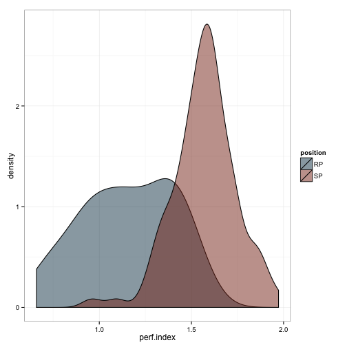
And then the the distributions for whip and era, respectively:
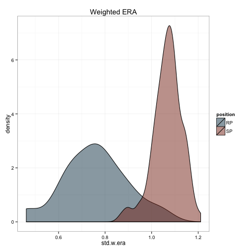
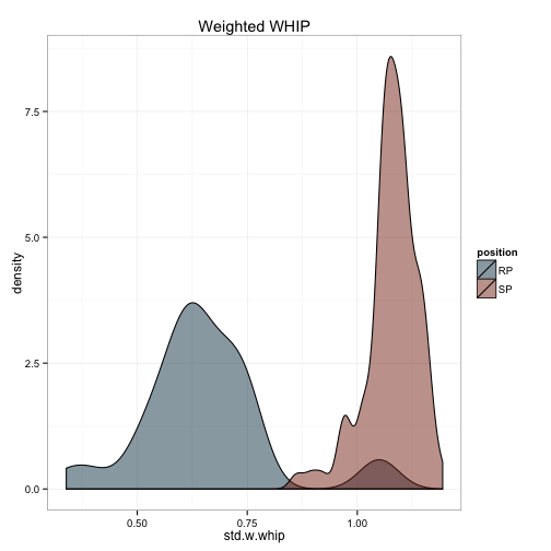
This is the basis for the rankings:
\[PI = Z_log(win) + Z_save + Z_log(k) + Z_w.era + Z_w.whip\]Where $PI$ is the performance index, and each term represents the standardized value of the average prediction from each projection system. The terms for $w.era$ and $w.whip$ are calculated as:
\[w.era = ERA * (predicted innings/\mu_predicted innings)\]and
\[w.whip = WHIP * (predicted innings/\mu_predicted innings)\]This seems to punish relievers more than you would expect. After all, a 1.86 ERA from Aroldis Chapman is certainly going to help your fantasy team more than the 4.17 ERA we’re expeting from Trevor Bauer. However, Chapman also pitches fewer innings, meaning his 1.86 ERA is not going to be as meaningful as an equivalent ERA from a starter.
I did some digging to see if anyone else had done something similar, and behold, someone had a different solution which seeems to make some sense:
The innings pitched constant was derived by finding the average innings pitched per start (total IP / GS), which was 5.94 from 2009-2011. Multiply that by 32.4—the average number of starts per pitcher in a five-man rotation (162 divided by 5)—which equals 192.5
So, my new weighting formulas are:
\[w.era = ERA * (predicted innings/192.5)\] \[w.whip = WHIP * (predicted innings/192.5)\]##Pitching stats
pit$agg.sd.w <- apply(pit[,c('fans_W', 'steamer_W', 'zips_W')], 1, function(x)
sd(x, na.rm=T))
#zips doesn't forecast saves
pit$agg.sd.sv <- apply(pit[,c('fans_SV', 'steamer_SV')], 1, function(x) sd(x, na.rm=T))
pit$agg.sd.k <- apply(pit[,c('fans_SO', 'steamer_SO', 'zips_SO')], 1, function(x)
sd(x, na.rm=T))
pit$agg.sd.era <- apply(pit[,c('fans_ERA', 'steamer_ERA', 'zips_ERA')], 1,
function(x) sd(x, na.rm=T))
pit$agg.sd.whip <- apply(pit[,c('fans_WHIP', 'steamer_WHIP', 'zips_WHIP')], 1,
function(x) sd(x, na.rm=T))
bat$agg.pa <- apply(bat[,c('fans_PA', 'steamer_PA', 'zips_PA')], 1,
function(x) mean(x, na.rm=T))
pit$agg.ip <- apply(pit[,c('fans_IP', 'steamer_IP', 'zips_IP')], 1,
function(x) mean(x, na.rm=T))
bat$agg.sd.pa <- apply(bat[,c('fans_PA', 'steamer_PA', 'zips_PA')], 1,
function(x) sd(x, na.rm=T))
pit$agg.sd.ip <- apply(pit[,c('fans_IP', 'steamer_IP', 'zips_IP')], 1,
function(x) sd(x, na.rm=T))
bat$agg.pa[bat$agg.pa == 1] <- NA
bat$pa.weight <- bat$agg.pa/mean(bat$agg.pa, na.rm=T)
pit$agg.ip[pit$agg.ip == 1] <- NA
pit$ip.weight <- pit$agg.ip/192.5
pit <- pit[pit$agg.k > 1,]
pit$agg.w[pit$agg.w==0] <- .5
log.w <- log(pit$agg.w)
pit$agg.w.std <- scale(log.w)
pit$agg.sv.std <- NA
pit$agg.sv.std[which(pit$agg.sv > 0)] <- scale(pit$agg.sv[which(pit$agg.sv > 0)])
#logged because of the skew
pit$agg.k.std <- scale(log(pit$agg.k))
pit$agg.era.std <- scale(pit$agg.era)*-1
pit$agg.whip.std <- scale(pit$agg.whip)*-1
pit$agg.w.era.std <- scale(pit$agg.era)*pit$ip.weight*-1
pit$agg.w.whip.std <- scale(pit$agg.whip)*pit$ip.weight*-1
pit$talent.index <- rowSums(pit[,c(72:74, 77,78)], na.rm=T)
pit.length <- length(pit$fans_Name)
bat.length <- length(bat$fans_Name)
combined <- data.frame(name=c(as.character(pit$fans_Name), as.character(bat$fans_Name)),
perf.index=c(scale(pit$talent.index), scale(bat$talent.index)),
std.w=c(pit$agg.w.std, rep(NA, bat.length)),
std.sv=c(pit$agg.sv.std, rep(NA, bat.length)),
std.k=c(pit$agg.k.std, rep(NA, bat.length)),
std.w.era=c(pit$agg.w.era.std, rep(NA, bat.length)),
std.w.whip=c(pit$agg.w.whip.std, rep(NA, bat.length)),
std.era=c(pit$agg.era.std, rep(NA, bat.length)),
std.whip=c(pit$agg.whip.std, rep(NA, bat.length)),
std.r=c(rep(NA, pit.length), bat$agg.runs.std),
std.hr=c(rep(NA, pit.length), bat$agg.hr.std),
std.rbi=c(rep(NA, pit.length), bat$agg.rbi.std),
std.sb=c(rep(NA, pit.length), bat$agg.sb.std),
std.obp=c(rep(NA, pit.length), bat$agg.obp.std),
std.w.obp=c(rep(NA, pit.length), bat$agg.w.obp.std),
ip=c(pit$agg.ip, rep(NA, bat.length)),
w=c(pit$agg.w, rep(NA, bat.length)),
sv=c(pit$agg.sv, rep(NA, bat.length)),
k=c(pit$agg.k, rep(NA, bat.length)),
era=c(pit$agg.era, rep(NA, bat.length)),
whip=c(pit$agg.whip, rep(NA, bat.length)),
pa=c(rep(NA, pit.length), bat$agg.pa),
r=c(rep(NA, pit.length), bat$agg.runs),
hr=c(rep(NA, pit.length), bat$agg.hr),
rbi=c(rep(NA, pit.length), bat$agg.rbi),
sb=c(rep(NA, pit.length), bat$agg.sb),
obp=c(rep(NA, pit.length), bat$agg.obp),
w.obp=c(rep(NA, pit.length), bat$agg.w.obp)
)
library(rvest)
library(stringr)
library(car)
url <- html('http://fantasynews.cbssports.com/fantasybaseball/rankings/h2h/overall/yearly')
pos <- url %>%
html_nodes('td:nth-child(1) td+ td') %>%
html_text()
POS <- str_extract(pos, "\\(\\w{1,2}\\)")
name <- str_extract(pos, perl(".*(?=\\s.{1,3}\\()"))
POS <- gsub('\\(', '', POS)
POS <- gsub('\\)', '', POS)
df.id <- data.frame(name = name,
position = as.factor(POS))
df.id$position <- recode(df.id$position, "c('LF', 'RF', 'CF')='OF'")
df <- full_join(df.id, combined)## Joining by: "name"## Warning: joining factors with different levels, coercing to character
## vectordf.pit <- subset(df, df$position=='SP' | df$position=='RP')
df.bat <- df[-grep('.P', df$position), ]
rownames(df.pit) <- 1:nrow(df.pit)
rownames(df.bat) <- 1:nrow(df.bat)
df.pit<-arrange(df.pit, desc(perf.index))The new result? Here’s the top 50:
df.pit[1:50, c(1:3, 17:22)]## name position perf.index ip w sv
## 1 Clayton Kershaw SP 4.620183 220.33333 17.333333 0.0
## 2 Felix Hernandez SP 3.856482 218.76667 15.000000 0.0
## 3 Max Scherzer SP 3.665071 209.10000 16.000000 0.0
## 4 Chris Sale SP 3.619888 203.23333 14.333333 0.0
## 5 Madison Bumgarner SP 3.565212 211.33333 15.000000 0.0
## 6 Corey Kluber SP 3.416722 210.76667 15.000000 0.0
## 7 Stephen Strasburg SP 3.393162 197.10000 14.333333 0.0
## 8 David Price SP 3.203842 218.23333 15.333333 0.0
## 9 Johnny Cueto SP 3.173662 196.43333 14.333333 0.0
## 10 Adam Wainwright SP 3.118677 200.90000 15.000000 0.0
## 11 Zack Greinke SP 3.117751 195.00000 14.000000 0.0
## 12 Jordan Zimmermann SP 3.066845 198.43333 14.000000 0.0
## 13 Jon Lester SP 3.056568 210.56667 14.333333 0.0
## 14 Cole Hamels SP 2.960434 210.66667 11.666667 0.0
## 15 James Shields SP 2.870500 210.23333 12.000000 0.0
## 16 Julio Teheran SP 2.831175 205.33333 13.000000 0.0
## 17 Masahiro Tanaka SP 2.830515 178.33333 12.666667 0.0
## 18 Matt Harvey SP 2.756780 167.66667 10.333333 0.0
## 19 Hisashi Iwakuma SP 2.714421 187.00000 12.333333 0.0
## 20 Alex Cobb SP 2.688449 189.56667 12.333333 0.0
## 21 Hyun-Jin Ryu SP 2.600947 174.76667 12.666667 0.0
## 22 Phil Hughes SP 2.549979 199.43333 13.666667 0.0
## 23 Gerrit Cole SP 2.521233 179.23333 12.666667 0.0
## 24 Sonny Gray SP 2.517992 205.33333 13.666667 0.0
## 25 Lance Lynn SP 2.513550 195.23333 14.000000 0.0
## 26 Alex Wood SP 2.471718 178.43333 11.000000 0.0
## 27 Aroldis Chapman RP 2.455834 63.66667 4.333333 36.0
## 28 Tyson Ross SP 2.401124 180.56667 11.666667 0.0
## 29 Jeff Samardzija SP 2.398521 204.33333 11.666667 0.0
## 30 Doug Fister SP 2.378225 183.76667 12.333333 0.0
## 31 Garrett Richards SP 2.370496 164.00000 11.333333 0.0
## 32 Matt Shoemaker SP 2.341373 178.00000 12.333333 0.0
## 33 Kenley Jansen RP 2.340722 67.66667 4.000000 37.0
## 34 Homer Bailey SP 2.329180 183.90000 10.666667 0.0
## 35 Jacob deGrom SP 2.324287 176.76667 10.666667 0.0
## 36 Craig Kimbrel RP 2.304146 64.10000 3.666667 36.5
## 37 Gio Gonzalez SP 2.287172 173.43333 11.666667 0.0
## 38 Justin Verlander SP 2.280238 207.43333 14.000000 0.0
## 39 Francisco Liriano SP 2.261729 168.90000 12.000000 0.0
## 40 Jake Arrieta SP 2.259024 169.43333 11.000000 0.0
## 41 Drew Smyly SP 2.253994 152.23333 10.333333 0.0
## 42 Carlos Carrasco SP 2.206929 158.33333 10.000000 0.0
## 43 Ian Kennedy SP 2.202069 191.90000 11.000000 0.0
## 44 Anibal Sanchez SP 2.198909 160.33333 11.333333 0.0
## 45 Collin McHugh SP 2.198552 176.90000 11.333333 0.0
## 46 Greg Holland RP 2.186108 65.00000 3.666667 37.5
## 47 Danny Salazar SP 2.178595 155.66667 10.666667 0.0
## 48 John Lackey SP 2.177320 181.56667 12.000000 0.0
## 49 Jered Weaver SP 2.142984 184.66667 13.000000 0.0
## 50 Jose Fernandez SP 2.136093 118.33333 8.333333 0.0
## k era whip
## 1 245.33333 2.283333 0.9700000
## 2 227.00000 2.750000 1.0600000
## 3 241.66667 2.896667 1.0833333
## 4 228.66667 2.850000 1.0633333
## 5 210.33333 2.886667 1.0866667
## 6 225.33333 3.033333 1.1133333
## 7 220.66667 2.996667 1.0833333
## 8 212.00000 3.380000 1.1166667
## 9 179.33333 2.963333 1.1200000
## 10 169.33333 3.040000 1.1300000
## 11 183.66667 2.990000 1.1300000
## 12 168.33333 3.116667 1.1133333
## 13 197.00000 3.156667 1.1666667
## 14 202.66667 3.270000 1.1466667
## 15 185.66667 3.280000 1.1600000
## 16 181.00000 3.336667 1.1600000
## 17 169.33333 3.260000 1.1000000
## 18 172.33333 3.023333 1.1100000
## 19 154.66667 3.350000 1.1200000
## 20 171.66667 3.170000 1.1900000
## 21 155.33333 3.256667 1.1566667
## 22 169.00000 3.696667 1.1633333
## 23 170.66667 3.380000 1.1900000
## 24 175.33333 3.383333 1.2500000
## 25 183.66667 3.366667 1.2533333
## 26 169.66667 3.273333 1.2000000
## 27 107.00000 1.863333 0.9466667
## 28 175.00000 3.286667 1.2433333
## 29 196.00000 3.726667 1.2133333
## 30 130.00000 3.353333 1.1933333
## 31 151.33333 3.233333 1.1966667
## 32 149.33333 3.596667 1.1766667
## 33 98.33333 2.306667 0.9633333
## 34 162.66667 3.556667 1.1900000
## 35 164.33333 3.446667 1.2033333
## 36 97.66667 2.000000 0.9533333
## 37 172.33333 3.436667 1.2400000
## 38 177.00000 3.796667 1.2500000
## 39 176.00000 3.363333 1.2666667
## 40 165.00000 3.470000 1.2166667
## 41 142.00000 3.330000 1.1633333
## 42 155.33333 3.470000 1.1833333
## 43 187.00000 3.693333 1.2500000
## 44 144.00000 3.496667 1.1933333
## 45 165.33333 3.656667 1.2200000
## 46 90.00000 2.273333 1.0100000
## 47 171.66667 3.640000 1.1933333
## 48 149.66667 3.693333 1.2166667
## 49 143.00000 3.783333 1.2200000
## 50 131.66667 2.906667 1.1200000Looks much better to me! Just to check, here’s those distributions:
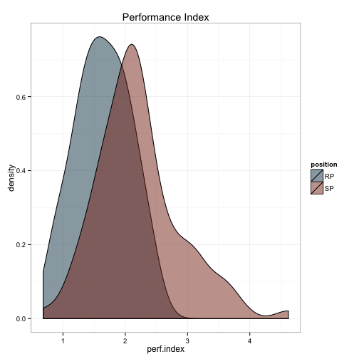
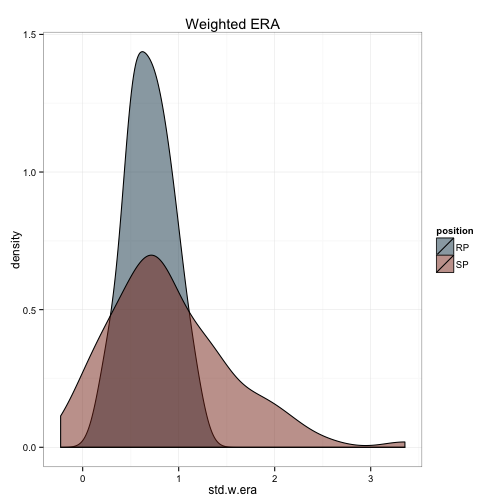
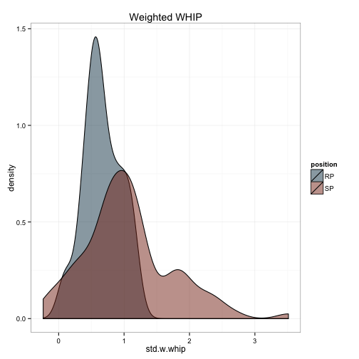
This looks much better and is what I used when I went into draft day.
What’s the lesson here? I guess that its wise to look to others before trying to reinvent the wheel. I should have known that someone had already tried an approach similar to mine. Stand on the shoulders of giants, as well as regular folks, and, for that matter, anyone else who is around. Just make sure you give proper credit where it’s due.