
Nested Nutrition
Recall that I’ve described the menustat.org data in a couple of previous posts. One of the first things I decided to do with it was to investigate what should be a pretty lawful set of relationships - that between the three primary macronutrients and total calories. Each macronutrient contain a set number of calories per gram:
- Fats: 9 kcal/gram
- Protiens: 4 kcal/gram
- Carbohydrates: 4 kcal/gram
This implies that if we predict the number of calories in the collection of food listed in our menustat data from the listed macronutrients, then we should obtain regression coefficients which are just about equal to those numbers (e.g. the regression coefficient for fats should be nearly exactly 9). Is this true? I’ve skipped the reading and cleaning of data, as I’ve covered it extensively elsewhere.
menus<-readLines('../Data/menustat-546cf6b433804.csv')
menus<-menus[-1]
menus<-gsub('\t-', '', menus)
menus<-gsub('\t', '', menus)
menus<-read.csv(textConnection(menus)) #this takes a minute...
submenus<-menus[,3:51] #leave 'Restuarant', 'Food Category', and 'Menu Item ID' untouched.
submenus[]<-lapply(submenus, as.character)
menus[,3:51]<-submenus

submenus<-menus[,c(7:15, 19:51)]
submenus[]<-lapply(submenus, as.numeric)
menus[,c(7:15, 19:51)]<-submenus

library(reshape2)
library(stringr)
library(plyr)
df <- melt(menus, id.vars = c('Restaurant.', 'Food.Category.', 'Item_Name.',
                           'Menu_Item_ID'))
df$year <- df$variable
levels(df$year) <- str_match(levels(df$variable), "[0-9]{4}")
levels(df$variable) <- gsub('\\.{1,2}', '', levels(df$variable))#remove dots
levels(df$variable) <- gsub('[0-9]', '', levels(df$variable))#remove year
levels(df$variable) <- gsub('\\s+$', '', levels(df$variable))#remove trailing space
df<-dcast(df, Restaurant. + Food.Category. + Item_Name. + Menu_Item_ID + year ~
           variable , value.var = 'value')
df<-arrange(df, Restaurant., Item_Name.)
df$Carbohydratesg[131161] <- NA
df[75620, 16] <- 300
df[75620, 21] <- 3
df[75815, 16] <- 250
df[75815, 21] <- 3
df[122305,12] <- NA
df[122305,11] <- NA
df$Calories <- as.numeric(df$Calories)
df$Proteing <- as.numeric(df$Proteing)
df$TotalFatg <- as.numeric(df$TotalFatg)
df$Carbohydratesg <- as.numeric(df$Carbohydratesg)
###Always looking at data### As might be clear by now, I’m a big advocate of looking at data first, before modeling anything. So, let’s scatter the things we’re interested in modeling:
library(ggplot2)
ggplot(df, aes(x=Proteing, y=Calories)) +
  geom_point(color='#88301B') +
  theme_bw()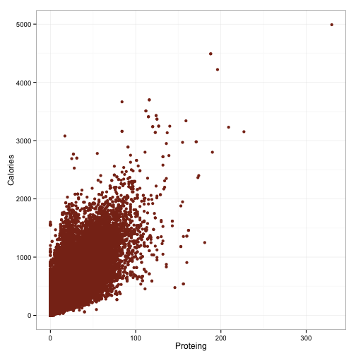
ggplot(df, aes(x=TotalFatg, y=Calories)) +
  geom_point(color='#88301B') +
  theme_bw()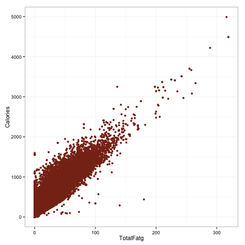
ggplot(df, aes(x=Carbohydratesg, y=Calories)) +
  geom_point(color='#88301B') +
  theme_bw()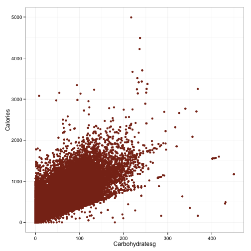
So that’s pretty interesting. Although these are certainly strong relationships, the mapping is not perfect. There is, however, a pretty hard cutoff for each of these things. The upward spread in each can probably be accounted for by the other macronutrients. Points which fall along the hard cutoff will be foods that contain only the macronutrient illustrated in that plot, because having 100 grams of protein but only 5 calories is not possible. However, haivng 100 grams of protein and 2000 calories certainly is.
###Simple model### As a first pass, let’s account for all this observed variability in a simple linear model.
m.1 <- lm(Calories~Proteing + Carbohydratesg + TotalFatg, data=df)
summary(m.1)
##
## Call:
## lm(formula = Calories ~ Proteing + Carbohydratesg + TotalFatg,
## data = df)
##
## Residuals:
## Min 1Q Median 3Q Max
## -1615.00 -6.02 -0.99 5.37 722.36
##
## Coefficients:
## Estimate Std. Error t value Pr(>|t|)
## (Intercept) 2.955325 0.159318 18.55 <2e-16 ***
## Proteing 4.163968 0.008474 491.40 <2e-16 ***
## Carbohydratesg 3.825203 0.002970 1287.99 <2e-16 ***
## TotalFatg 8.989266 0.007465 1204.24 <2e-16 ***
## ---
## Signif. codes: 0 '***' 0.001 '**' 0.01 '*' 0.05 '.' 0.1 ' ' 1
##
## Residual standard error: 30.88 on 92728 degrees of freedom
## (87982 observations deleted due to missingness)
## Multiple R-squared: 0.9919, Adjusted R-squared: 0.9919
## F-statistic: 3.767e+06 on 3 and 92728 DF, p-value: < 2.2e-16Hey! That’s almost perfect! The coefficients for proteins and carbs are not significantly different than 4, and the coefficient for fat is not significantly different than 9 - just like you would expect for something dictated by a lawful relationship such as this. Moreover, the r-squared is an astonishing .99. Wow. I’ve never analyzed anything like this before.
However, they’re not exactly right, are they. In fact, there’s something that caught my eye here. It’s the direction of the estimates. When Americans look at the nutrition of the food they’re consuming, do you think that, in general, they’re looking to maximize or minimize their intake of protein? What about carbohydrates? And fat?
Do you notice that the direction that each of these estimates differ from zero go in precisely the same direction as the social desireability of each macronutrient? Maybe this is nothing - just noise in the data that happens to correspond to some broader social issue. Or, maybe it isn’t.
###Clustered Data### One thing we can do is see if there are individual eateries whose reported nutritional info is systematically in line with these societal expectancies. This also highlights a major problem with using a standard linear model in this situation - our data are clustered. There are lots of ways in which this is true, but one obvious one is that it is clustered by restaurant. This means that the observations from one restaruant are going to look more like the observations from that restaurant than they will observations from another restaurant. This structure violates one of the assumptions of the simple linear model I ran above. One way around this is to use a mixed effects model.
library(lme4)
names(df)[1] <- 'Restaurant'
m.2 <- lmer(Calories ~ Proteing + Carbohydratesg + TotalFatg +
       (1+Proteing+Carbohydratesg+TotalFatg|Restaurant), data=df)
## Warning in checkConv(attr(opt, "derivs"), opt$par, ctrl = control$checkConv, : Model is nearly unidentifiable: very large eigenvalue
## - Rescale variables?summary(m.2)## Linear mixed model fit by REML ['lmerMod']
## Formula:
## Calories ~ Proteing + Carbohydratesg + TotalFatg + (1 + Proteing +
## Carbohydratesg + TotalFatg | Restaurant)
## Data: df
##
## REML criterion at convergence: 883964.3
##
## Scaled residuals:
## Min 1Q Median 3Q Max
## -40.725 -0.215 0.000 0.207 25.233
##
## Random effects:
## Groups Name Variance Std.Dev. Corr
## Restaurant (Intercept) 159.05823 12.6118
## Proteing 0.58292 0.7635 -0.10
## Carbohydratesg 0.08753 0.2959 -0.53 -0.18
## TotalFatg 0.48318 0.6951 -0.03 -0.81 -0.16
## Residual 791.12562 28.1270
## Number of obs: 92732, groups: Restaurant, 145
##
## Fixed effects:
## Estimate Std. Error t value
## (Intercept) 4.53776 1.07887 4.21
## Proteing 4.18548 0.06578 63.63
## Carbohydratesg 3.82201 0.02542 150.37
## TotalFatg 8.90414 0.05983 148.83
##
## Correlation of Fixed Effects:
## (Intr) Protng Crbhyd
## Proteing -0.101
## Carbhydrtsg -0.526 -0.178
## TotalFatg -0.032 -0.800 -0.159That kicked out a nasty warning message (which seems to be because of the size of the dataset). I could scale the variables to get rid of it, but everything seems to look okay (note the coefficient estimate), so I’ll just move forward.
The basic idea here is that we’ve fit a model which is largely similar to the first one, but allowed the intercept and effects of protein, carbohydrate, and fat to randomly vary by restaurant. Now that we’ve done this, we can go in and get these random effects to see how restaurants may differ in their reported relationship between these macronutrients and the calories. I’m going to get these values and standardize them. This will allow me to ignore the fact that there’s probably going to be more variability on fat because it’s got a higher mean value. I’m also going to reverse the direction of the values for protein because I want the values for each of these to be consistent with social desireability. In other words, it is socially desireable to indicate lower numbers for carbohydrates and total fat, but higher numbers for protein. I’m going to switch the sign on protein so that for all three, lower numbers mean more socially desireable.
Question of interest: What happens if I standardize the random effects versus standardize the predictors in the model?
rf <- ranef(m.2)
df.rf <- rf$Restaurant
head(df.rf)
## (Intercept) Proteing Carbohydratesg TotalFatg
## 7 Eleven -0.8866613 -0.03064419 0.138203380 -0.074145871
## A&W -0.9205591 1.39110394 -0.007611939 -1.239607760
## Applebee's -6.0821036 -0.32458787 0.078870370 0.211500580
## Arby's -3.1506740 -0.26323209 -0.040117254 0.399496869
## Au Bon Pain -2.4939369 0.23708863 -0.087233413 -0.021850158
## Auntie Anne's -3.6354658 0.35671209 0.131298041 0.003991585df.rf$Proteing <- scale(df.rf$Proteing)
df.rf$Proteing <- df.rf$Proteing*-1
df.rf$Carbohydratesg <- scale(df.rf$Carbohydratesg)
df.rf$TotalFatg <- scale(df.rf$TotalFatg)Now, let’s look at the deviation on these bad boys. We can sum across each random effect to examine a new metric I’m going to call ‘reporting tendency’. Negative numbers here will indicate a tendency to report in a socially desireable way, while positive numbers will indicate a tendency to report in a non-socially desireable way.
df.rf$reporting.tendency <- df.rf$Proteing + df.rf$Carbohydratesg +
  df.rf$TotalFatg
ggplot(df.rf, aes(x=reporting.tendency)) +
  geom_histogram(binwidth=.2, fill='#144256') +
  theme_bw() + ylab('Count') + xlab('Reporting Tendency')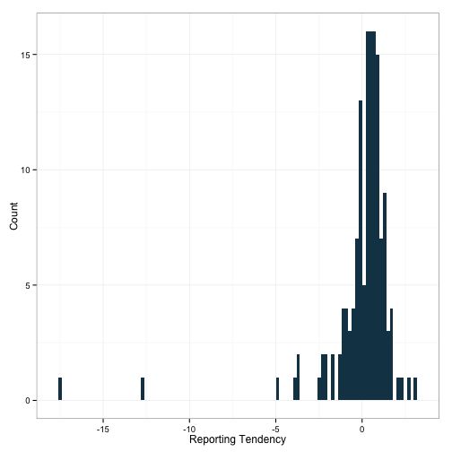
Hm. A couple of outliers down there. This whole exercise may yet end up being another lesson in what messy data is really like. I’m going to have to address this in a future post.
How’s that for a cliffhanger?