
Modeling Horoscope Language, Part 2
This is a continuation of a series of blog posts in which I work with some horoscopes I scraped from the New York Posts’s website. In the last post, I showed that the language didn’t really contain any information that would allow us to identify which sign the particular horoscope came from. However, that doesn’t mean the language doesn’t contain any information.
Conveniently, we also have the publication date for each horoscope. Not only that, but there are also 12 months of the year, just as there are 12 astrological signs. This means that it is easy and straightforward to compare how well we can classify on zodiac sign (not well at all) with how well we can classify on the month of the year.
First, let’s pull out just the month of the year from our data.
import pandas as pd
df = pd.read_csv('./../data/astrosign.csv', sep='|')
df = df.drop('Unnamed: 0', 1)
df=df.dropna()
df['month'] = df['pub_date'].map(lambda x: str(x)[0:2])
df.head()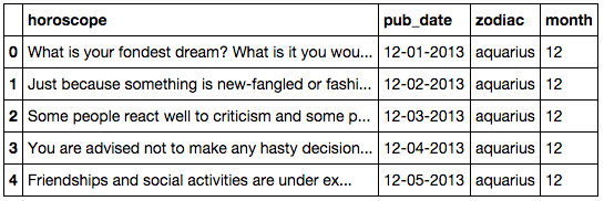
Now, we can repeat our classification procedure with this new set of labels that indicate the month in which the horoscope was written.
from sklearn.feature_extraction.text import CountVectorizer
from sklearn.cross_validation import train_test_split
from sklearn import svm

cv = CountVectorizer()
wordcounts = cv.fit_transform(df['horoscope'])
scope_train, scope_test, month_train, month_true = \
    train_test_split(wordcounts,
                     df.month,
                     test_size=.3,
                     random_state=42)

clf = svm.LinearSVC()
clf.fit(scope_train, month_train)
## LinearSVC(C=1.0, class_weight=None, dual=True, fit_intercept=True,
## intercept_scaling=1, loss='l2', multi_class='ovr', penalty='l2',
## random_state=None, tol=0.0001, verbose=0)from sklearn import metrics
predicted = clf.predict(scope_test)
scores = metrics.classification_report(month_true, predicted)
print scores## precision recall f1-score support
##
## 01 0.32 0.33 0.33 203
## 02 0.35 0.33 0.34 210
## 03 0.31 0.37 0.34 207
## 04 0.27 0.33 0.30 190
## 05 0.28 0.26 0.27 186
## 06 0.32 0.32 0.32 117
## 07 0.31 0.21 0.25 126
## 08 0.24 0.26 0.25 108
## 09 0.37 0.28 0.32 113
## 10 0.35 0.30 0.33 102
## 11 0.32 0.29 0.31 102
## 12 0.31 0.31 0.31 218
##
## avg / total 0.31 0.31 0.31 1882HA! We know more about the month of the year than we do about the astrological sign being discussed. Man my job is cool.
Just in case you don’t remember (or you never looked), here’s what this classification would look like if there was no real relationship between the horoscope and the month it was published. We can establish this by just shuffling the labels such that they are randomly paired with horoscopes rather than paired with the one that they truly belong with.
import numpy as np
df['shuffled_month'] = np.random.permutation(df.month)
df.head()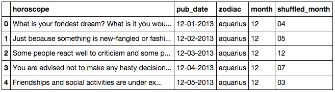
scope_train, scope_test, month_train, month_true = \
    train_test_split(wordcounts,
                     df['shuffled_month'],
                     test_size=.3,
                     random_state=42)

clf = svm.LinearSVC()
clf.fit(scope_train, month_train)
predicted = clf.predict(scope_test)
scores = metrics.classification_report(month_true, predicted)
print scores
## precision recall f1-score support
##
## 01 0.13 0.12 0.13 233
## 02 0.15 0.15 0.15 191
## 03 0.16 0.15 0.16 237
## 04 0.08 0.09 0.08 194
## 05 0.08 0.09 0.09 173
## 06 0.02 0.03 0.03 96
## 07 0.03 0.03 0.03 117
## 08 0.11 0.09 0.10 108
## 09 0.10 0.08 0.09 123
## 10 0.04 0.03 0.03 98
## 11 0.06 0.05 0.05 96
## 12 0.10 0.12 0.11 216
##
## avg / total 0.10 0.10 0.10 1882I would say that this pretty convincingly shows that there’s more information in the horoscopes that pertains to the month of the year in which it was published than the astrological sign.
Just to be complete, let’s use a random forest as well, just like we tried in the last post.
from sklearn.ensemble import RandomForestClassifier

#the RF classifier doesn't take the sparse numpy array we used before,
#so we just have to turn it into a regular array. This doesn't change
#the values at all, it just changes the internal representation.
wcarray = wordcounts.toarray()

scope_train, scope_test, month_train, month_true = \
    train_test_split(wcarray,
                     df.month,
                     test_size=.3,
                     random_state=42)

clf = RandomForestClassifier()
clf.fit(scope_train, month_train)
predicted = clf.predict(scope_test)
scores = metrics.classification_report(month_true, predicted)
print scores
## precision recall f1-score support
##
## 01 0.22 0.47 0.30 203
## 02 0.28 0.36 0.32 210
## 03 0.25 0.38 0.30 207
## 04 0.25 0.32 0.28 190
## 05 0.26 0.23 0.25 186
## 06 0.54 0.27 0.36 117
## 07 0.55 0.21 0.31 126
## 08 0.48 0.21 0.29 108
## 09 0.60 0.27 0.37 113
## 10 0.59 0.25 0.36 102
## 11 0.46 0.23 0.30 102
## 12 0.39 0.28 0.33 218
##
## avg / total 0.37 0.31 0.31 1882A random forest seems to give us a bit better precision in this case, but the f1 score is the same. There’s a problem here, however. Unlike when we were using horoscopes, our classes are not roughly equivalent in terms of the number of instances. Specifically, there are fewer cases for the months of June through November. This could be (and almost certainly is) biasing our learner and is an important factor to consider when fitting these kinds of models.