In a previous post, I started investigating the number of publications in Scopus as a function of specific search terms (e.g. affect). Even before getting started, I noticed something that looked like an artifact in the data. Specifically, there was a large jump in the number of publications from 1995 to 1996. I spent some time doing a little more digging and thought I’d post an update on this.

Although I could obtain search results going back well before the turn of the century, I made the decision, for this portion of investigation, to focus only on the 90’s. I obtained search results from 1990 to 2000. However, rather than retrieving the data by specific search terms, I opted to obtain the number of publications by year and journal. My rationale was that the artifact might be a function of something weird going on with some subset of journals which suddenly rapidly increased the number of articles they published.

The result of these searches was one csv file for each year. There were two data columns - one indicating the source (i.e. journal), and one indicating the number of papers from that year for that journal. Here’s what I did:

Import needed modules:

import pandas as pd
import re
import glob
import os
import matplotlib.pyplot as plt

Now, load in the files:

pathdir = os.path.dirname(os.path.abspath('__file__'))
pathdir = os.chdir('..')
files = glob.glob('data/Scopus-*.csv')
data = pd.DataFrame()
for f in files:
    yearfile = pd.read_csv(f, skiprows=7) #first 7 rows are not relevant
    year = re.search('[1-2][0-9][0-9][0-9]', f) #get the year from the filename
    yearfile['Year'] = year.group(0)
    data = pd.concat([data, yearfile])

As much as I like column names like ‘Unnamed: 1’, I think something a little less unique is in order:

data.rename(columns={'SOURCE TITLE':'Source Title', 'Unnamed: 1':'Papers'}, 
        inplace=True)

Okay, so now we’ve got something to work with. Just as a refresher, I’m looking to explain this weird jump from 1995 to 1996:

papersbyyear = data.groupby('Year')['Papers'].sum()
papersbyyear.plot()

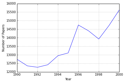
The first thing I thought to do was to see if perhaps there was just an increase in the number of journals. This could either be because Scopus started listing more journals in 1996, or because several journals were launched that year.

titlesbyyear = data.groupby('Year')['Source Title'].nunique()
ax=titlesbyyear.plot(ylim=(155,165))
ax.set_ylabel('Number of Journals')

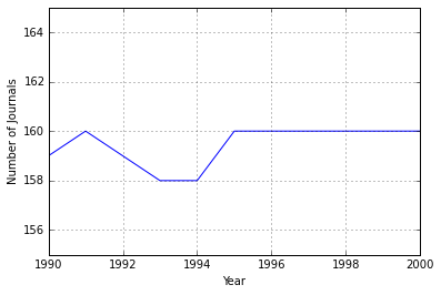
That’s a whole lot of nothing going on. The line is basically flat. To be totally honest, that line looks too flat to me. It seems like there should be more variation than that. Regardless, this can’t account for the jump we saw in the figure above.

The next stage was to examine how much journals changed from 1995 to 1996. Basically, I’m looking for the ratio of papers published in 1996 to papers published in 1995. The best way I know to do this is by moving some numbers around in the dataframe. The below turns it from long to wide. This will allow me to straightforwardly compute the ratio of the column for 1996 over the column for 1995:

datawide = data.groupby(['Year', 'Source Title']).Papers.sum().unstack('Year')
datawide['Change'] = datawide['1996']/datawide['1995'] 

Now to visualize these, let’s look at a histogram. Histograms are handy ways of quickly identifying if there are any obvious outliers, which is kind of what we’re doing here:

datawide['Source Title'] = datawide.index
data_long = pd.melt(datawide, id_vars=['Source Title', 'Change'])
plt.hist(data_long['Change'].dropna(), 35)

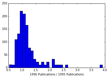
There’s one which exhibits a pretty big jump, and then a handful of others which also are increasing by more than a factor of 2. I’m going to look at just these “big movers”.

movers = data_long[data_long['Change'] > 2] #select the big movers
moversyearindex = movers.pivot(index='Year', columns='Source Title', 
                      values='value') #give each Journal its own column
#
#This is to make sure the plots appear in order from highest to lowest change
movers = movers[['Source Title', 'Change']]
movers = movers.drop_duplicates()
cols=movers['Source Title'].tolist()
moversyearindex = moversyearindex[cols]

Now plot each of these “big movers”. I tried to do the following with a loop, but it kept spitting out an error after only printing one plot (TypeError: 'instancemethod' object has no attribute '__getitem__'). What’s going on here is that I’ve made subplots for each of the journals (which each have their own column in the moversyearindex dataframe). After plotting each column, I then give each subplot it’s own title (e.g. axes[0].set_title(moversyearindex.columns.values[0])). There’s also a line to reduce the number of ticks on the y axis, as well as a line to clean up the layout (plt.tight_layout()).

fig, axes = plt.subplots(nrows=8, ncols=1, figsize=(8, 10), sharex=True, 
                         sharey=True)
yloc=plt.MaxNLocator(4)
moversyearindex[moversyearindex.columns.values[0]].plot(ax=axes[0])
axes[0].set_title(moversyearindex.columns.values[0])
axes[0].yaxis.set_major_locator(yloc)
moversyearindex[moversyearindex.columns.values[1]].plot(ax=axes[1])
axes[1].set_title(moversyearindex.columns.values[1])
moversyearindex[moversyearindex.columns.values[2]].plot(ax=axes[2])
axes[2].set_title(moversyearindex.columns.values[2])
moversyearindex[moversyearindex.columns.values[3]].plot(ax=axes[3])
axes[3].set_title(moversyearindex.columns.values[3])
moversyearindex[moversyearindex.columns.values[4]].plot(ax=axes[4])
axes[4].set_title(moversyearindex.columns.values[4])
moversyearindex[moversyearindex.columns.values[5]].plot(ax=axes[5])
axes[5].set_title(moversyearindex.columns.values[5])
moversyearindex[moversyearindex.columns.values[6]].plot(ax=axes[6])
axes[6].set_title(moversyearindex.columns.values[6])
moversyearindex[moversyearindex.columns.values[7]].plot(ax=axes[7])
axes[7].set_title(moversyearindex.columns.values[7])
plt.tight_layout()

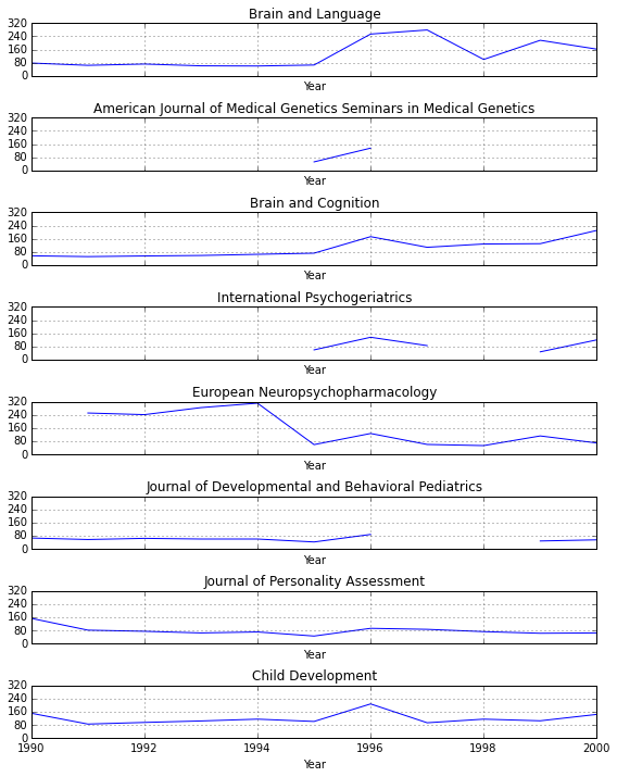
These are sorted from largest to smallest change. Where the lines don’t exist are years for which there are no data. Brain and Language is obviously the biggest changer. I went to the journal’s website to see if the numbers here roughly corresponded to what I could find there.

They didn’t. I was able to find 74 for 1995 and 112 for 1996. Nowhere near the 65 and 254, respectively, listed here.

At this point, I feel like this dataset is not really worth exploring. There’s got to be a better way to access academic article listings. Even so, it’s a bit worrying that the results given by Scopus appear to be pretty unreliable. This, I guess, is exhibit A for why one shouldn’t just rely on any solitairy search tool.

I’d still like to answer my original question, but until I find a more reliable data source, I think it’s going to have to be postponed.