
Plot and Clean
In a previous post, I described a dataset taken from menustat.org. I used the dataset to illustrate how some minor tweaks can get your analyses to run much more quickly.
Anyway, the data are interesting in its own right, so I thought I’d look at some of what’s in it here.
Menustat data
To refresh, the current dataset consists of over 180,000 observations, consisting of food items from 3 years (2014, 2013, and 2012). The variables indicate the restaurant which serves the food item, the category that item falls into (e.g. entree, appetizer, etc), the year, and then nutrition information. In this post, I’m going to make some preliminary plots, focusing on calories plus the macronutrients - carbs, proteins, and fats. For ease of examination, I’m going to plot these as a function of which food category they belong to.
library(ggplot2)
library(dplyr)
df$Calories <- as.numeric(df$Calories)
ordered.df <- group_by(df, Food.Category.) %>%
  summarise(med = median(Calories, na.rm=T)) %>%
  arrange(desc(med)) %>%
  as_data_frame()
df$Food.Category. <- factor(df$Food.Category., levels=ordered.df$Food.Category.)

plot <- ggplot(df, aes(x=Food.Category., y=Calories))
plot + geom_boxplot(fill='#ABC3CE') +
  xlab('Food Category') +
  theme_bw() +
  theme(axis.text.x = element_text(angle=15, vjust=.9))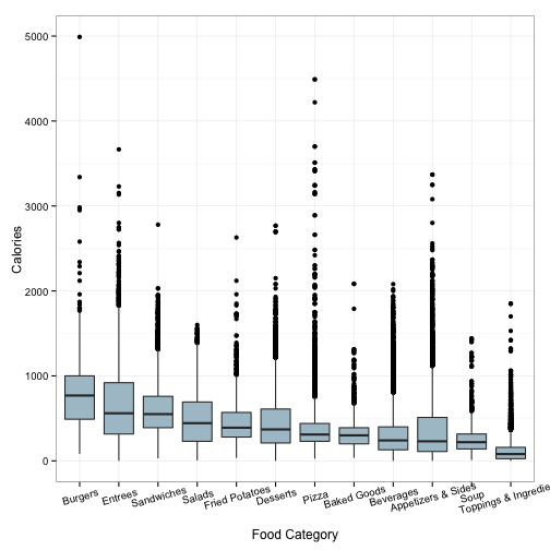
I’ve also taken the liberty of ordering the x axis according to median, descending from left to right. Nothing especially surprising here. Biggest calorie bombs are Burgers, Entrees, and Sandwiches. One Burger tips the scales at around 5000 calories, and while that’s around 2 days worth of the recommended daily energy needs for the average male, I guess it isn’t too surprising. This is the land of the free and home of the brave, after all. Next up is carbs:
df$Carbohydratesg <- as.numeric(df$Carbohydratesg)
ordered.df <- group_by(df, Food.Category.) %>%
  summarise(med = median(Carbohydratesg, na.rm=T)) %>%
  arrange(desc(med)) %>%
  as_data_frame()
df$Food.Category. <- factor(df$Food.Category., levels=ordered.df$Food.Category.)


plot <- ggplot(df, aes(x=Food.Category., y=Carbohydratesg))
plot + geom_boxplot(fill='#ABC3CE') +
  xlab('Food Category') + ylab('Carbohydrates') +
  theme_bw() +
  theme(axis.text.x = element_text(angle=15, vjust=.9))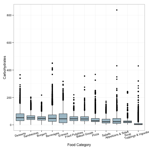
This is a bit odd. There’s apparently a side or appetizer which has north of 800 grams of carbohydrates. I find this hard to believe. Let’s look a little more closely.
subset(df, df$Carbohydratesg > 800)## Restaurant. Food.Category. Item_Name.
## 131161 Red Robin Appetizers & Sides Guacamole & Salsa w/ Chips
## Menu_Item_ID year ItemDescription
## 131161 51697 2014 Guacamole & Salsa w/ Chips, Appetizers
## ServingsPerItem ServingSize ServingSizeUnit ServingsSizeText
## 131161 <NA> <NA> <NA>
## Calories TotalFatg SaturatedFatg TransFatg Cholesterolmg Sodiummg
## 131161 313 36 <NA> <NA> <NA> 1239
## Potassiummg Carbohydratesg Fiberg Sugarg Proteing
## 131161 <NA> 838 10 5 8Ah! My old alma mater! I spent about 7 months employed by Red Robin in the year between undergrad and my master’s program at SFSU. It let me pay off the absurd costs incurred by applying to graduate school in my first attempt. Anyway, this seems to say that there are 838 grams of carbohydrates in 313 calories worth of Guac & Salsa with chips. I don’t know that I believe this. Let’s look at the rows around it (where the same item for 2013 and 2012 should appear)
df[131161:131163,]## Restaurant. Food.Category. Item_Name.
## 131161 Red Robin Appetizers & Sides Guacamole & Salsa w/ Chips
## 131162 Red Robin Appetizers & Sides Guacamole & Salsa w/ Chips
## 131163 Red Robin Appetizers & Sides Guacamole & Salsa w/ Chips
## Menu_Item_ID year ItemDescription
## 131161 51697 2014 Guacamole & Salsa w/ Chips, Appetizers
## 131162 51697 2013 Guacamole & Salsa w/ Chips, Appetizers
## 131163 51697 2012
## ServingsPerItem ServingSize ServingSizeUnit ServingsSizeText
## 131161 <NA> <NA> <NA>
## 131162 <NA> 204 <NA>
## 131163 <NA> <NA> <NA>
## Calories TotalFatg SaturatedFatg TransFatg Cholesterolmg Sodiummg
## 131161 313 36 <NA> <NA> <NA> 1239
## 131162 555 31 <NA> <NA> <NA> 1008
## 131163 NA <NA> <NA> <NA> <NA> <NA>
## Potassiummg Carbohydratesg Fiberg Sugarg Proteing
## 131161 <NA> 838 10 5 8
## 131162 <NA> 63 10 4 7
## 131163 <NA> NA <NA> <NA> <NA>Well, 2013 seems to be about as expected. 2014, however, seems to be a lost cause. I even did a bit of poking around on the web to see if I could find some better information, but there doesn’t seem to be anything on the first page or two of google. We’ll replace these carb count here with NA and replot.
df$Carbohydratesg[131161] <- NA
plot <- ggplot(df, aes(x=Food.Category., y=Carbohydratesg))
plot + geom_boxplot(fill='#ABC3CE') +
  xlab('Food Category') + ylab('Carbohydrates') +
  theme_bw() +
  theme(axis.text.x = element_text(angle=15, vjust=.9))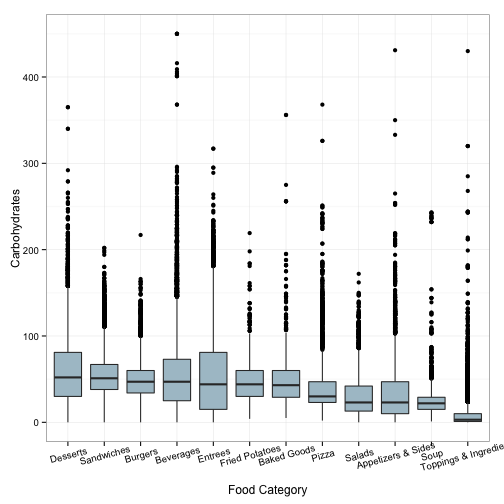
That’s much better. On to protein:
df$Proteing <- as.numeric(df$Proteing)
ordered.df <- group_by(df, Food.Category.) %>%
  summarise(med = median(Proteing, na.rm=T)) %>%
  arrange(desc(med)) %>%
  as_data_frame()
df$Food.Category. <- factor(df$Food.Category., levels=ordered.df$Food.Category.)

plot <- ggplot(df, aes(x=Food.Category., y=Proteing))
plot + geom_boxplot(fill='#ABC3CE') +
  xlab('Food Category') + ylab('Protein') +
  theme_bw() +
  theme(axis.text.x = element_text(angle=15, vjust=.9))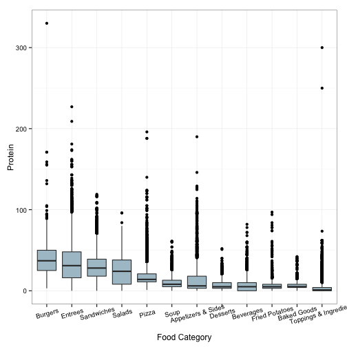
Okay, a few oddities. A couple of `Toppings & Ingredients’ with quite a bit more protein than one would think. Also, there’s a burger with over 300 grams of protein. I’ll bet it’s the one with 5000 calories.
subset(df, df$Proteing > 240)## Restaurant. Food.Category.
## 75620 Hungry Howie's Pizza Toppings & Ingredients
## 75815 Hungry Howie's Pizza Toppings & Ingredients
## 93469 Max & Erma's Burgers
## Item_Name. Menu_Item_ID year
## 75620 Blue Cheese Dressing, Sauces 45084 2013
## 75815 Ranch Dressing 45083 2013
## 93469 Landfill Burger 69763 2014
## ItemDescription ServingsPerItem ServingSize
## 75620 Blue Cheese Dressing, Sauces <NA> 28
## 75815 Ranch Dressing, Sauces <NA> 28
## 93469 Landfill Burger, Burgers <NA> <NA>
## ServingSizeUnit ServingsSizeText Calories TotalFatg SaturatedFatg
## 75620 <NA> 152 1 1
## 75815 <NA> 175 1 0
## 93469 <NA> 4990 316 108
## TransFatg Cholesterolmg Sodiummg Potassiummg Carbohydratesg Fiberg
## 75620 <NA> 16 3 <NA> 20 0
## 75815 <NA> 19 3 <NA> 3 0
## 93469 13 1050 7760 <NA> 217 19
## Sugarg Proteing
## 75620 <NA> 300
## 75815 <NA> 250
## 93469 30 330First of all, behold the Landfill Burger. Yikes. That is the definition of an outlier. Still, I see no reason to remove it or anything. That’s a real thing. A real burger.
Moving on, we see the sides of Blue Cheese and Ranch dressing. Popular among body builders as a quick dose of protein immediately following a workout…
Except not at all. Let’s first try to correct these two observations by looking at the neighboring rows.
df[75619:75621,]## Restaurant. Food.Category.
## 75619 Hungry Howie's Pizza Toppings & Ingredients
## 75620 Hungry Howie's Pizza Toppings & Ingredients
## 75621 Hungry Howie's Pizza Toppings & Ingredients
## Item_Name. Menu_Item_ID year
## 75619 Blue Cheese Dressing, Sauces 45084 2014
## 75620 Blue Cheese Dressing, Sauces 45084 2013
## 75621 Blue Cheese Dressing, Sauces 45084 2012
## ItemDescription ServingsPerItem ServingSize
## 75619 Blue Cheese Dressing, Sauces <NA> 28
## 75620 Blue Cheese Dressing, Sauces <NA> 28
## 75621 <NA> <NA>
## ServingSizeUnit ServingsSizeText Calories TotalFatg SaturatedFatg
## 75619 <NA> 152 1 1
## 75620 <NA> 152 1 1
## 75621 <NA> NA <NA> <NA>
## TransFatg Cholesterolmg Sodiummg Potassiummg Carbohydratesg Fiberg
## 75619 <NA> 16 300 <NA> 20 0
## 75620 <NA> 16 3 <NA> 20 0
## 75621 <NA> <NA> <NA> <NA> NA <NA>
## Sugarg Proteing
## 75619 <NA> 3
## 75620 <NA> 300
## 75621 <NA> NAOkay, I think we can safely correct that value of 300 grams of protein to a 3. While we’re at it, we can also fix the sodium figure for the same year.
df[75620, 16] <- 300
df[75620, 21] <- 3
For ranch dressing:
df[75814:75816,]## Restaurant. Food.Category. Item_Name.
## 75814 Hungry Howie's Pizza Toppings & Ingredients Ranch Dressing
## 75815 Hungry Howie's Pizza Toppings & Ingredients Ranch Dressing
## 75816 Hungry Howie's Pizza Toppings & Ingredients Ranch Dressing
## Menu_Item_ID year ItemDescription ServingsPerItem ServingSize
## 75814 45083 2014 Ranch Dressing, Sauces <NA> 28
## 75815 45083 2013 Ranch Dressing, Sauces <NA> 28
## 75816 45083 2012 <NA> <NA>
## ServingSizeUnit ServingsSizeText Calories TotalFatg SaturatedFatg
## 75814 <NA> 175 1 0
## 75815 <NA> 175 1 0
## 75816 <NA> NA <NA> <NA>
## TransFatg Cholesterolmg Sodiummg Potassiummg Carbohydratesg Fiberg
## 75814 <NA> 19 250 <NA> 3 0
## 75815 <NA> 19 3 <NA> 3 0
## 75816 <NA> <NA> <NA> <NA> NA <NA>
## Sugarg Proteing
## 75814 <NA> 3
## 75815 <NA> 250
## 75816 <NA> NASame problem! Someone switched the numbers somewhere.
df[75815, 16] <- 250
df[75815, 21] <- 3
Replot:
plot <- ggplot(df, aes(x=Food.Category., y=Proteing))
plot + geom_boxplot(fill='#ABC3CE') +
  xlab('Food Category') + ylab('Protein') +
  theme_bw() +
  theme(axis.text.x = element_text(angle=15, vjust=.9))
Okay, that’s much better. Last, let’s look at fat:
df$TotalFatg <- as.numeric(df$TotalFatg)
ordered.df <- group_by(df, Food.Category.) %>%
  summarise(med = median(TotalFatg, na.rm=T)) %>%
  arrange(desc(med)) %>%
  as_data_frame()
df$Food.Category. <- factor(df$Food.Category., levels=ordered.df$Food.Category.)


plot <- ggplot(df, aes(x=Food.Category., y=TotalFatg))
plot + geom_boxplot(fill='#ABC3CE') +
  xlab('Food Category') + ylab('Total Fat') +
  theme_bw() +
  theme(axis.text.x = element_text(angle=15, vjust=.9))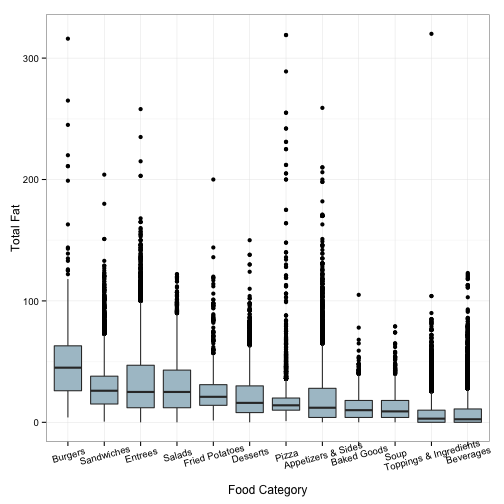
One more offender in toppings & ingredients.
subset(df, df$TotalFatg > 300)## Restaurant. Food.Category.
## 93469 Max & Erma's Burgers
## 122311 Pollo Tropical Toppings & Ingredients
## 167323 Unos Pizza
## 167324 Unos Pizza
## Item_Name.
## 93469 Landfill Burger
## 122311 Yellow Rice w/ Vegetables, for Create Your Own TropiChop Bowl
## 167323 Chicago Classic, Deep Dish Pizza, Regular
## 167324 Chicago Classic, Deep Dish Pizza, Regular
## Menu_Item_ID year
## 93469 69763 2014
## 122311 51018 2014
## 167323 56105 2014
## 167324 56105 2013
## ItemDescription
## 93469 Landfill Burger, Burgers
## 122311 Yellow Rice w/ Vegetables, for Create Your Own TropiChop Bowl, Regular, Base Items
## 167323 Chicago Classic, Deep Dish Pizza w/ Sausage, Mozzarella, Chunky Tomato Sauce & Romano, Regular
## 167324 Chicago Classic, Deep Dish Pizza, Regular
## ServingsPerItem ServingSize ServingSizeUnit ServingsSizeText
## 93469 <NA> <NA> <NA>
## 122311 <NA> <NA> <NA>
## 167323 <NA> 1475 <NA>
## 167324 <NA> 1475 <NA>
## Calories TotalFatg SaturatedFatg TransFatg Cholesterolmg Sodiummg
## 93469 4990 316 108 13 1050 7760
## 122311 10 320 5 <NA> 1 830
## 167323 4490 319 101 1.5 430 9540
## 167324 4490 319 101 1.5 430 9540
## Potassiummg Carbohydratesg Fiberg Sugarg Proteing
## 93469 <NA> 217 19 30 330
## 122311 <NA> 64 4 1 7
## 167323 <NA> 237 9 16 188
## 167324 <NA> 237 9 16 188Yeah, no way a yellow rice & veg bowl has 320 grams of fat.
df[122305:122307,]## Restaurant. Food.Category.
## 122305 Pollo Tropical Appetizers & Sides
## 122306 Pollo Tropical Appetizers & Sides
## 122307 Pollo Tropical Appetizers & Sides
## Item_Name. Menu_Item_ID year
## 122305 Yellow Rice w/ Vegetables, Meal Sides Choice of 2 50893 2014
## 122306 Yellow Rice w/ Vegetables, Meal Sides Choice of 2 50893 2013
## 122307 Yellow Rice w/ Vegetables, Meal Sides Choice of 2 50893 2012
## ItemDescription ServingsPerItem
## 122305 Yellow Rice w/ Vegetables, Meal Sides <NA>
## 122306 Yellow Rice w/ Vegetables, Meal Sides Choice of 2 <NA>
## 122307 <NA>
## ServingSize ServingSizeUnit ServingsSizeText Calories TotalFatg
## 122305 142 <NA> 160 3
## 122306 142 <NA> 160 3
## 122307 <NA> <NA> NA NA
## SaturatedFatg TransFatg Cholesterolmg Sodiummg Potassiummg
## 122305 0 <NA> 0 420 <NA>
## 122306 0 <NA> 0 420 <NA>
## 122307 <NA> <NA> <NA> <NA> <NA>
## Carbohydratesg Fiberg Sugarg Proteing
## 122305 32 2 0 4
## 122306 32 2 0 4
## 122307 NA <NA> <NA> NALooks like the calories and the fat here are both entered incorrectly. I’m tempted to make both of them the same as what is found on row 122306 (i.e. 320 calories, 5 grams of fat), but row 122306 specifies in the item description that the item is 10 ounces. There’s no such description in the offending row. So, I think I’ll just remove these mis-entered numbers.
df[122305,12] <- NA
df[122305,11] <- NA
replot:
plot <- ggplot(df, aes(x=Food.Category., y=TotalFatg))
plot + geom_boxplot(fill='#ABC3CE') +
  xlab('Food Category') + ylab('Total Fat') +
  theme_bw() +
  theme(axis.text.x = element_text(angle=15, vjust=.9))
Our variables of interest are now relatively clean, and we can proceed with some more interesting analyses. This will be the subject of a subsequent post.